2.5. Contaminant Transport and Pollution in Rivers

Another major challenge in groundwater systems is the transport of contaminants, that is something (potentially toxic) is released into the subsurface and travels with the groundwater, appearing in the water supply or a river at some point later in time (depending on the hydraulic conductivity of the aquifer, and the hydraulic head difference driving the flow). In some respects we have learned the tools you would need to determine how long before a contaminant released into the groundwater would be seen at some point downstream. You could figure out the lines of equipotential, and the hydraulic conductivity, and then calculate the flow velocity, and this would yield time (with some knowledge of the distance travelled). Here we are going to discuss how the contaminant plume evolves in the groundwater system.

Contaminant Transport in Groundwater

Having understood a bit about how the broader chemistry of groundwater evolves along the flow path, we can consider what happens when we add a contaminant to groundwater and how it is likely to travel and disperse through the groundwater system.

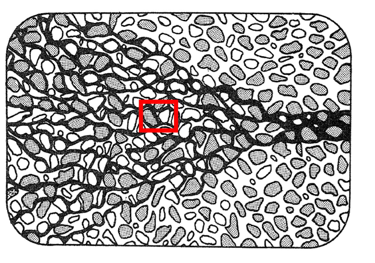
Fig. 2.36 A control volume in groundwater showing solute transport by advection and dispersion, with possible chemical reactions within the box.

If we consider a control volume in the groundwater where we have flow of a contaminant (or molecule or element – here we will call it a ‘solute’, meaning a component dissolved in groundwater) through that volume, we can apply mass conservation to this box. Solute can move into the box or out of the box, and chemical reactions can create or destroy solute within the box (e.g. mineral dissolution or precipitation). This allows us to consider the net rate of change of the concentration of the solute within the box.

So how does the solute, or contaminant, move through the control volume?

It moves by advection, and by dispersion.

Advection

Advection causes the wholesale movement of the solute with the flow field at the same velocity as the flow field. So if we have a solute (like a contaminant) in groundwater, and the groundwater is moving at a velocity of 5 metres per year, then if we return one year later, we expect the contaminant to have moved 5 metres away.

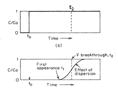
Fig. 2.37 The effect of advection on contaminant movement over time from \(t_0\) to \(t_2\), showing the displacement of the solute plume with the groundwater flow.

Fig. 2.37 shows the effect of advection on the movement of a contaminant over time from \(t_0\) to \(t_2\).

In reality what we find is that over this time we often get more than just the movement of the contaminant in the flow field but also the spreading out of the concentration. This is the effect of diffusion and hydrodynamic dispersion.

Dispersion

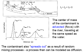
Fig. 2.38 Illustration of dispersion processes showing how a contaminant plume spreads due to molecular diffusion and mechanical dispersion.

Dispersion comprises molecular diffusion and mechanical dispersion; together these are called hydrodynamic dispersion.

• Molecular Diffusion describes the spread of particles through random motion from regions of higher concentration to regions of lower concentration. It is governed by Fick’s First law, where the overall flux due to molecular diffusion is given by a diffusion coefficient (determined in the lab) and the concentration gradient:

  (2.25)\[J = -D \pdv{C}{x}\]

  where \(J\) is the diffusive flux, \(D\) is the diffusion coefficient, and \(\pdv{C}{x}\) is the concentration gradient.

• Mechanical Dispersion reflects the fact that not everything in the porous medium travels at the average water flow speed. Some paths are faster, some slower, some longer, some shorter. This results in a net spreading of the solute plume that looks very much like a diffusive behaviour.

  

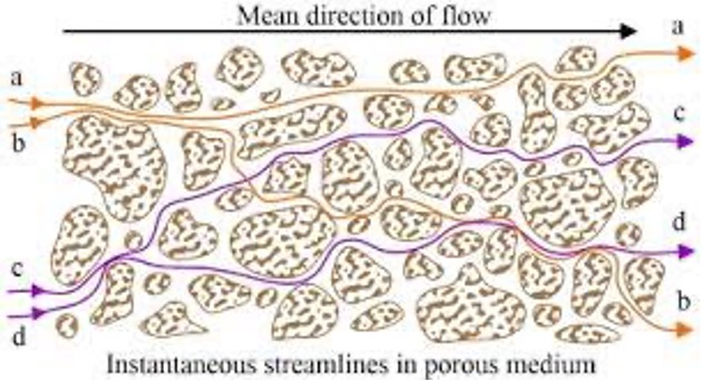
  Fig. 2.39 Modelling of the mechanical dispersion in porous media, showing variations in flow paths through the pore structure.

  Since mechanical dispersion depends on the flow, it is expected to increase with increasing flow speed. The most common expression for mechanical dispersion is given by:

  (2.26)\[D_m = \alpha v\]

  where \(D_m\) is the mechanical dispersion coefficient, \(\alpha\) is the dispersivity (units m, a property of the porous medium that grows with the scale of observation), and \(v\) is the average linear velocity. The total hydrodynamic dispersion coefficient is \(D = \alpha v + D^*\), where \(D^*\) is the effective molecular diffusion coefficient in the porous medium.

Note that given the very slow rate of molecular diffusion, advection and mechanical dispersion tend to dominate contaminant transport in groundwater.

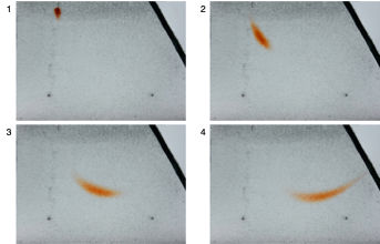
Fig. 2.40 Summary diagram showing the combined effects of advection, dispersion, and chemical reactions on contaminant transport in groundwater.

Chemical Reactions

• When solutes flow through a porous medium they can interact with the solid phase. In particular they can sorb and desorb, or precipitate into mineral phases, or dissolve into the groundwater from mineral phases.

• The amount of these chemical reactions and how they impact the overall chemical transport depends on the solute, water chemistry, and geochemical makeup of the porous medium.

The Advection-Dispersion Equation

Having discussed advection, dispersion, and chemical reactions individually, we can now consider how they combine in a mathematical framework.

We will not go through the mathematics of these models in detail, but the standard formula is:

Units!

\[\begin{split} C &= \mathrm{amount~m^{-3}} \\ D &= \mathrm{m^2~s^{-1}} \\ v &= \mathrm{m~s^{-1}} \\ R &= \mathrm{unitless} \end{split}\]

(2.27)\[R \frac{\partial C}{\partial t} = D \frac{\partial^2 C}{\partial x^2} - v \frac{\partial C}{\partial x}\]

Here \(D\) is the hydrodynamic dispersion coefficient and \(v\) the average linear velocity. \(R\) is the retardation factor, which accounts for sorption onto the solid phase: \(R = 1\) for a non-reactive tracer that moves with the water, and \(R > 1\) for a solute that sorbs and is therefore slowed relative to the water.

Where \(C\) is the contaminant concentration, and we are interested in how its concentration changes with time \(\left( \frac{\partial C}{\partial t} \right)\) and with distance \(\left( \frac{\partial C}{\partial x} \right)\). Because there are changes with time and with distance, we need to use a partial differential equation.

A solution for this is given by the equation below, which shows the concentration of a contaminant some distance from where it was released as a function of the overall flow velocity and the dispersion.

(2.28)\[C(x,y,z,t) = \frac{M}{n (4 \pi t)^{3/2} \sqrt{D_x D_y D_z}} \exp{\left[- \left( \frac{(x - v_x t)^2}{4 D_x t} + \frac{y^2}{4 D_y t} + \frac{z^2}{4 D_z t}\right) \right]}\]

where \(M\) is the mass of contaminant released instantaneously at the origin at \(t = 0\), \(n\) is the porosity, \(v_x\) is the average linear velocity in the \(x\) direction, and \(D_x\), \(D_y\), \(D_z\) are the dispersion coefficients in each direction. This assumes uniform flow in \(x\) and no sorption.

Extension: Navier-Stokes Equations (Non-Examinable)

Building on what we have discussed about hydraulic head in groundwater, we can consider the Navier-Stokes equations, which are partial differential equations that govern the motion of viscous fluids. These equations constitute the basic equations for fluid mechanics. They express conservation of momentum, and are solved together with conservation of mass (and, where heat matters, conservation of energy).

Conservation of mass means that mass in a control volume (basically a bit of the subsurface fluid – see Fig. 2.36) cannot be created or destroyed. Conservation of momentum means that momentum is not created or destroyed, and changes only because of forces acting on the control volume. Conservation of energy derives from the first law of thermodynamics: work and heat added to the system will result in an increase in the total energy of the system.

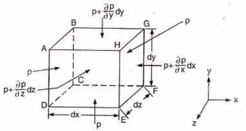
Fig. 2.41 A control volume showing the forces and momentum fluxes used in deriving the Navier-Stokes equations from conservation of momentum.

By understanding the forces on the control volume, we can derive partial differential equations that explain how fluids move through the control volume. The derivation of the Navier-Stokes equations is something we consider in QCES.

In beadpacks in the Institute for Energy and Environmental Flows you can see the stretching along the flowpath of an injection of dye (Fig. 2.42).

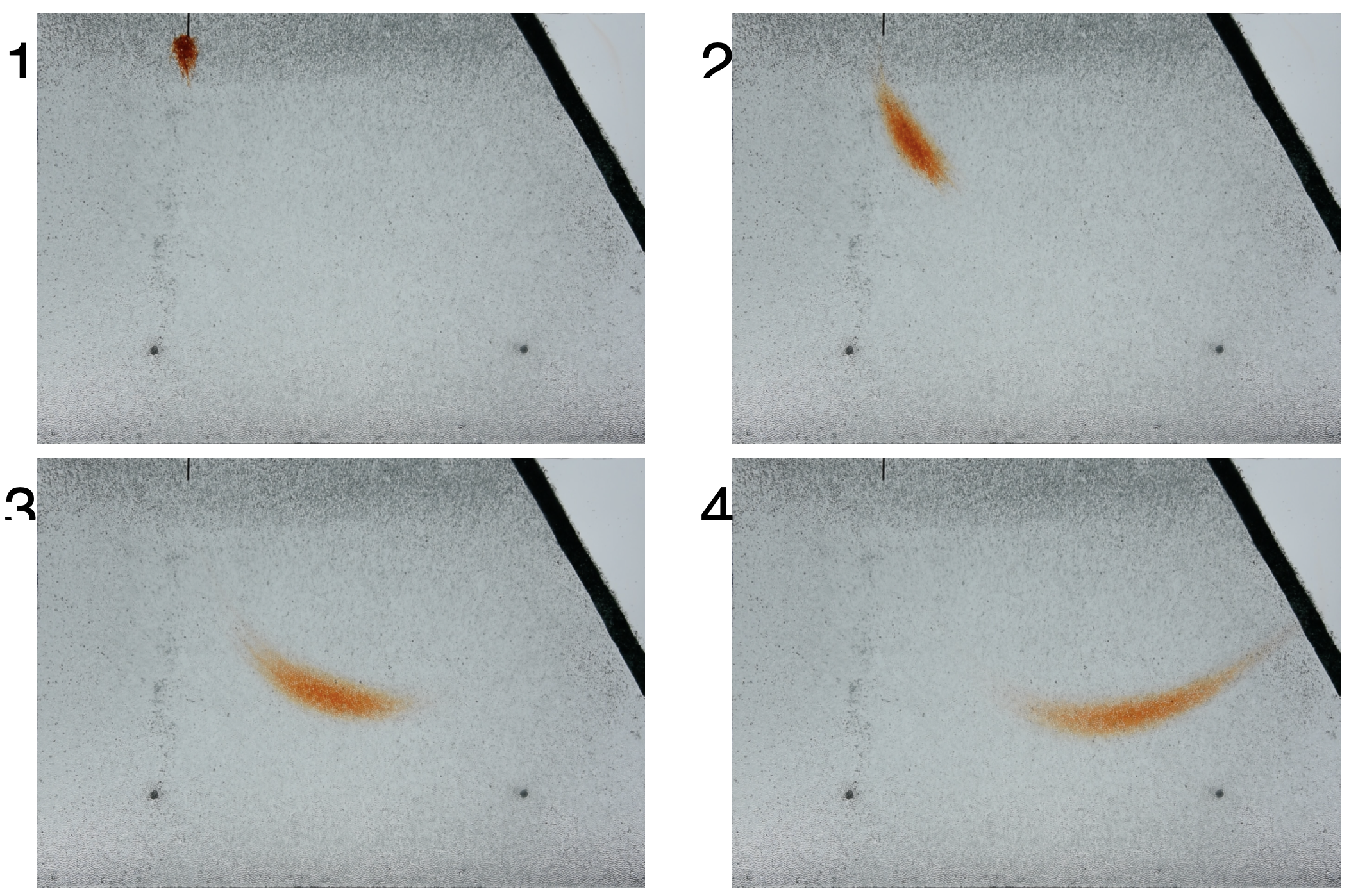
Fig. 2.42 Dye injection in a beadpack showing stretching along the flowpath.

The Péclet Number

Determining the relative importance of advection versus dispersion (so the growing shape of the contaminant plume during subsurface transport) is often done using the dimensionless Péclet Number (Fig. 2.43):

(2.29)\[\mathrm{Pe} = \frac{vL}{D}\]

where \(L\) is a characteristic length (often the grain size). When \(\mathrm{Pe} \gg 1\) advection dominates and the plume moves as a coherent body; when \(\mathrm{Pe} \ll 1\) dispersion dominates and the plume spreads out.

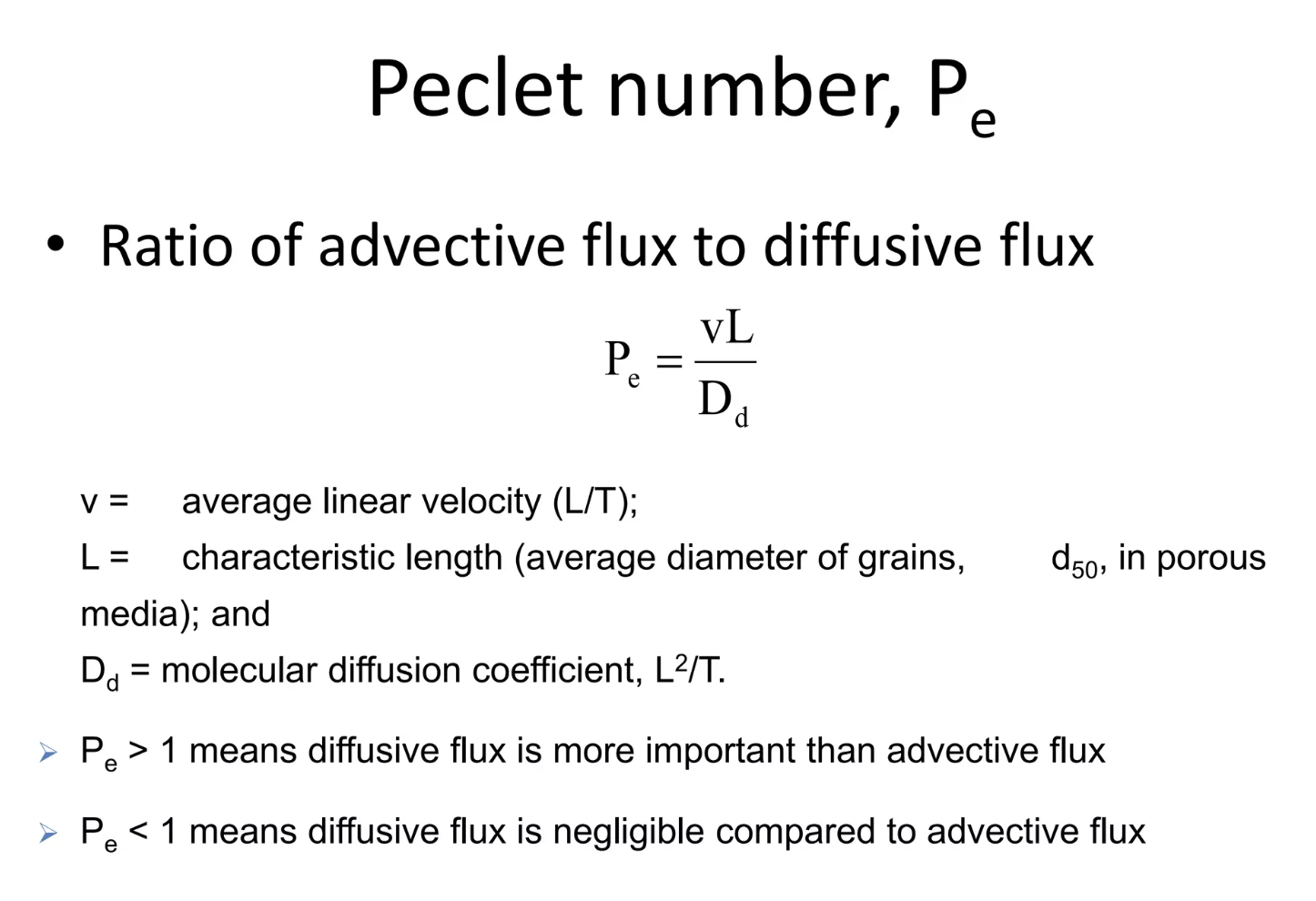
Fig. 2.43 The Péclet Number characterises the relative importance of advection and dispersion in contaminant transport.

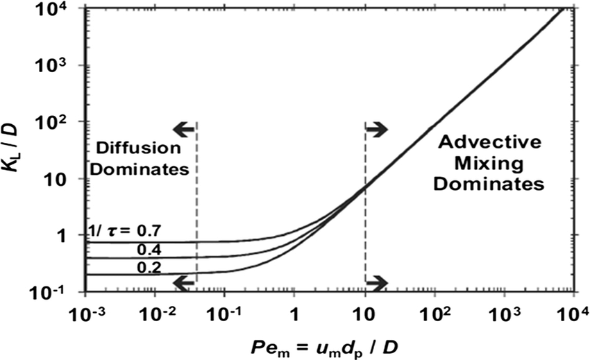
Fig. 2.44 Normalised dispersion coefficient plotted against Péclet number.

Contaminant Plume Modelling

If we assume that the contaminant spreads out in all directions as it moves along the flow of the groundwater, then we can track the shape of the contaminant plume away from the point source. Spreading in the \(x\) direction (along the flow) is controlled by longitudinal dispersion, while spreading in \(y\) and \(z\) is controlled by transverse dispersion, which is typically about an order of magnitude smaller, so plumes become elongated in the flow direction. With a series of simplifying assumptions (isotropic media, flow in the x direction etc.) we can use a Gaussian model to track plume movement over time (Fig. 2.45).

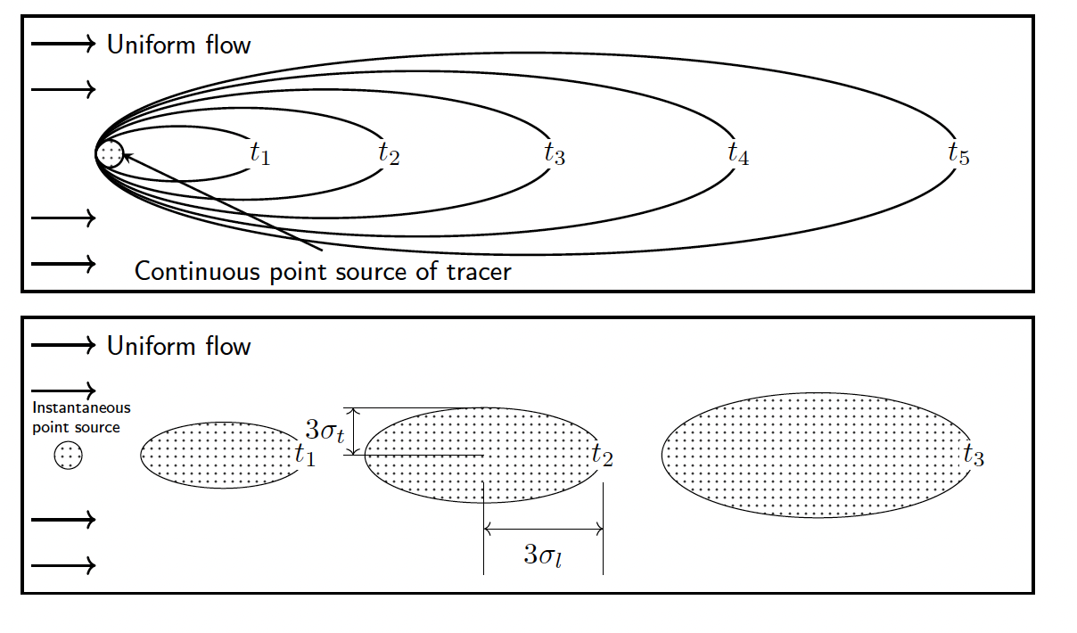
Fig. 2.45 Diagram showing the development of a contaminant plume in groundwater, tracking movement in three dimensions over time.

This is similar to the maths behind following a plume of smoke in the atmosphere (Fig. 2.46, Fig. 2.47).

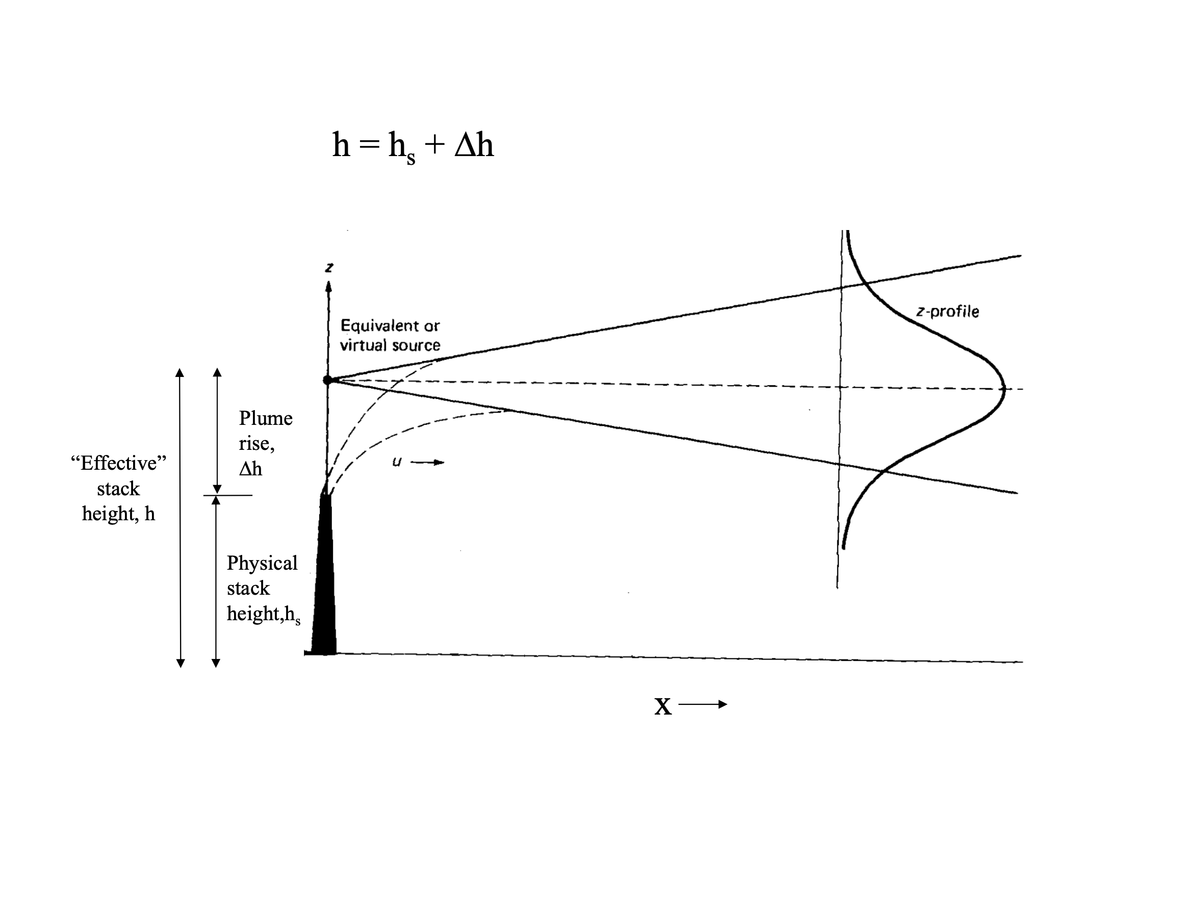
Fig. 2.46 A smoke plume in the atmosphere showing similar dispersion patterns.

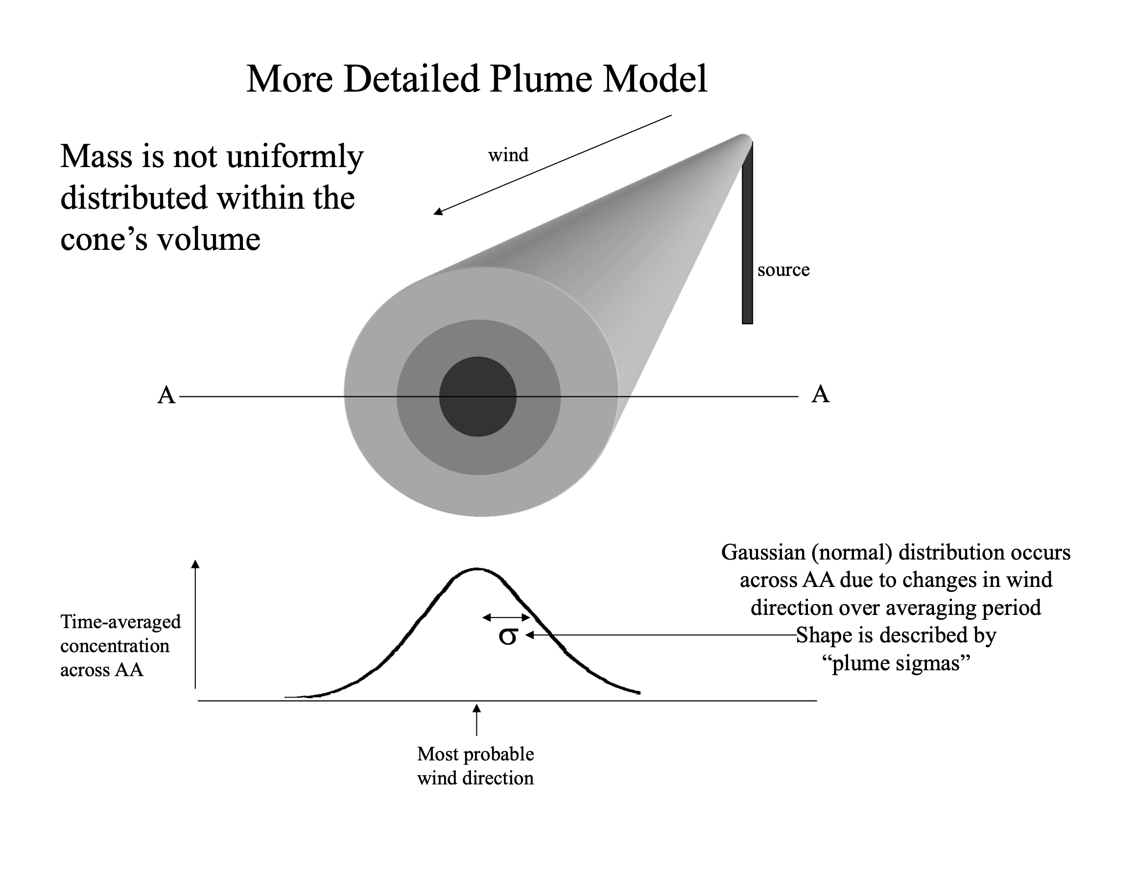
Fig. 2.47 Plume model diagram illustrating the mathematical framework for tracking dispersion.

Pollution in Rivers

Pollution in rivers has been a growing concern. In general, pollution in rivers is from the release of sewage, chemicals and nutrients into the rivers. The Rivers Trust has a bunch of maps that track pollution levels in rivers across the UK, including the amount of ‘forever chemicals’ (i.e. chemicals that are very hard to degrade so will stay in rivers for a very long time) and the rate of release of sewage. However, the largest source of pollution to rivers is through nutrients from agriculture.

Nutrients and Eutrophication

Nutrients refer largely to nitrate and phosphate, which are key macronutrients that are needed for photosynthesis. Nitrogen (in the form of ammonium or nitrate) is used in amino acids and proteins while phosphorus is used in DNA and RNA, ATP (the cell’s energy carrier) and the phospholipids of cell membranes. To get plants to grow you need a source of CO₂, water, light, nitrogen and phosphorus. This is why nitrogen and phosphorus are often added to soils in the form of fertilisers to maximise plant growth. UK farmers are subject to rules on fertiliser and manure use (e.g. Nitrate Vulnerable Zone regulations and, in England, the Farming Rules for Water), but enforcement is limited, so in practice cost is often the main constraint on how much fertiliser is applied.

As you add nitrogen and phosphorus run-off from agriculture to rivers you get growth of algae in the rivers, often measured as the chlorophyll abundance (Fig. 2.48).

Fig. 2.48 The addition of nitrate and phosphate leads to exceptional algal growth, shown by chlorophyll abundance.

When the algae die, their decomposition by bacteria consumes oxygen, depleting the water in oxygen. This sequence of nutrient enrichment, excess growth and oxygen depletion is eutrophication.

Fig. 2.49 The process of eutrophication: excess nutrients lead to algal blooms, which increase respiration and deplete oxygen levels in the water.

In the lecture we discussed the particular challenge of the River Wye, where intensification of poultry farming has increased phosphorus inputs, leading to widespread algal blooms and declining river health. Efforts to clean up rivers often focus on stemming the tide of runoff into the river. But much of the excess nutrient is stored in the landscape: nitrate leaches readily into groundwater, while phosphorus builds up in soils and is released slowly over years to decades (‘legacy’ nutrients). We can start to ask ourselves how long until it reaches the rivers and the challenges with eutrophication might be over?

Transit Time and Groundwater

The transit time simply might be considered:

(2.30)\[\text{Time} = \frac{\text{Length to travel}}{\text{velocity of fluid}}\]

Where the length might be how far a farm is from the river of interest and the velocity could be the rate of flow of a stream or the rate of flow of the groundwater derived from Darcy’s Law. For transport by advection alone, time scales linearly with length (\(t = L/v\)). In later lectures we will see why, for groundwater systems, the relevant timescale can instead scale with length² (as \(t \sim L^2/D\)), because of the flowpaths in the subsurface and the impact of dispersion.

Units!

\[\begin{split} \text{Time} &= \mathrm{s~or~yr} \\ \text{Length} &= \mathrm{m} \\ \text{velocity} &= \mathrm{m~s^{-1}} \end{split}\]

Groundwater and Surface Water Interactions

The take home from groundwater is the importance it plays in the overall surface water system!

Fig. 2.50 Diagram showing the network of interactions between groundwater and surface water systems.