7.3. The Biological Pump

Key Points:

• Phytoplankton grow in the ocean and take up CO₂ from the atmosphere via photosynthesis.

• The growth of phytoplankton is limited by the availability of nutrients and light.

• Phytoplankton fuel the marin food web, which produces organic matter in the surface.

• All this organic matter eventually sinks from the surface ocean.

• Sinking organic matter is ‘remineralised’ as it sinks, which releases dissolved C and nutrients back into the water.

• This exports carbon from the surface ocean to the deep, removing it from the atmosphere, and is known as the biological pump.

The surface ocean is a soup of microscopic life - one ml of average surface ocean water contains around 5 x 10⁵ organisms (and that estimate only includes prokaryotes!). Many of these organisms are photosynthetic phytoplankton, the ‘plants of the sea’, which harvest light energy from the sun to convert CO₂ into sugars. These are the ‘primary producers’ of the ocean, and are the base of the marine food web. Here, we’ll look at how the carbon trapped by these organisms is exported from the surface ocean to the deep, removing carbon from the atmosphere and concentrating it in the ocean.

Phytoplankton

Phytoplankton fuel a complex food web of zooplankton (Fig. 7.14), fish, and ultimately all marine life. However, for the purposes of understanding ocean carbon, we’re going to compress all this complexity to consider ‘organic matter’ - solid material that makes up the bodies of marine organisms that is created from dissolved CO₂ and light by phytoplankton. All organisms produce waste and eventually die, and this organic matter gradually sinks from the surface into the deep ocean. This constant rain of dead organisms and faecal matter from the surface ocean is known as marine snow, which makes it sound a lot nicer than it is!

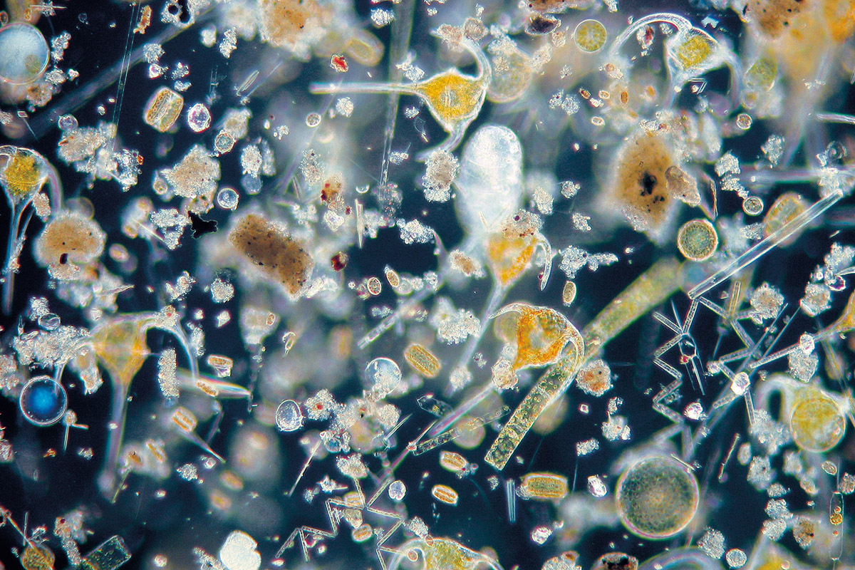
Fig. 7.14 A light micrograph of surface ocean plankton. This is typical of what you’d see down a microscope if you filtered a few litres of seawater. Most of the organisms you see here are zooplankton - micriscopic animals and the larval stages of larger organisms. The phytoplankton are the green- and brown-coloured particles you can see inside the zooplankton which have eaten them. Photo: Annegret Stuhr, GEOMAR.

Organic Matter

Organic matter is produced by phytoplankton from dissolved CO₂ in the ocean, and can be approximated as:

(7.17)\[\mathrm{\underbrace{6 CO_2}_{carbon~dioxide} + \underbrace{6 H_2O}_{water} \xrightarrow[+light]{photosynthesis} \underbrace{C_6H_{12}O_6}_{glucose} + \underbrace{6 O_2}_{oxygen}}\]

This describes the process of primary productivity in its most basic form: the capture of CO₂ from the atmosphere by photosynthesis, and the production of glucose, a simple sugar, which can fuel biological processes in organisms. This simplified reaction implies that photosynthesis only depends upon the presence of CO₂ and light; CO₂ is ubiquitously present in the surface ocean, so this would predict that photosynthesis should be capturing carbon from the atmosphere everywhere that there is light. We can see from Fig. 7.15 that this is not the case, with large regions of low productivity in the subtropical gyres, where there is abundant light.

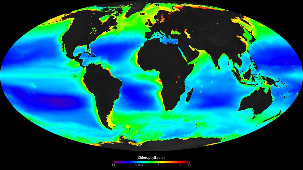
Fig. 7.15 The annual average concentration of chlorophyll in the surface ocean, as measured by the SeaWiFS satellite. Chlorophyll is the green pigment that phytoplankton use to harvest light energy, and its characteristic absorption spectrum make it possible to determine its concentration, and therefore phytoplankton abundance, from satellite measurements of ocean colour. Image from NASA.

Patterns of Productivity

Patterns in the abundance of phytoplankton are driven by the availability of nutrients and light, the two essential ingredients for photosynthesis. However, it is worth noting that while abundance varies greatly, phytoplankton are present everywhere in the surface ocean. Even the low chlorophyll regions in the subtropical guyres (Fig. 7.15) are home to a healthy population of particularly small phytoplankton that are specially adapted for living in these nutrient-poor waters. Some phytoplankton that live in polar oceans are able to survive the long winters, with almost no light for ~6 months.

The pervasive presence of phytoplankton throughout the surface ocean allows them to respond quickly to changes in the environment. A local upwelling of nutrient-rich waters caused by a storm or an eddy can trigger a phytoplankton bloom in the surface ocean (Fig. 7.16), as the local residents rapidly multiply to use up the available nutrients. This makes patterns of productivity much more ‘patchy’ than the annual average productivity that we see in Fig. 7.15.

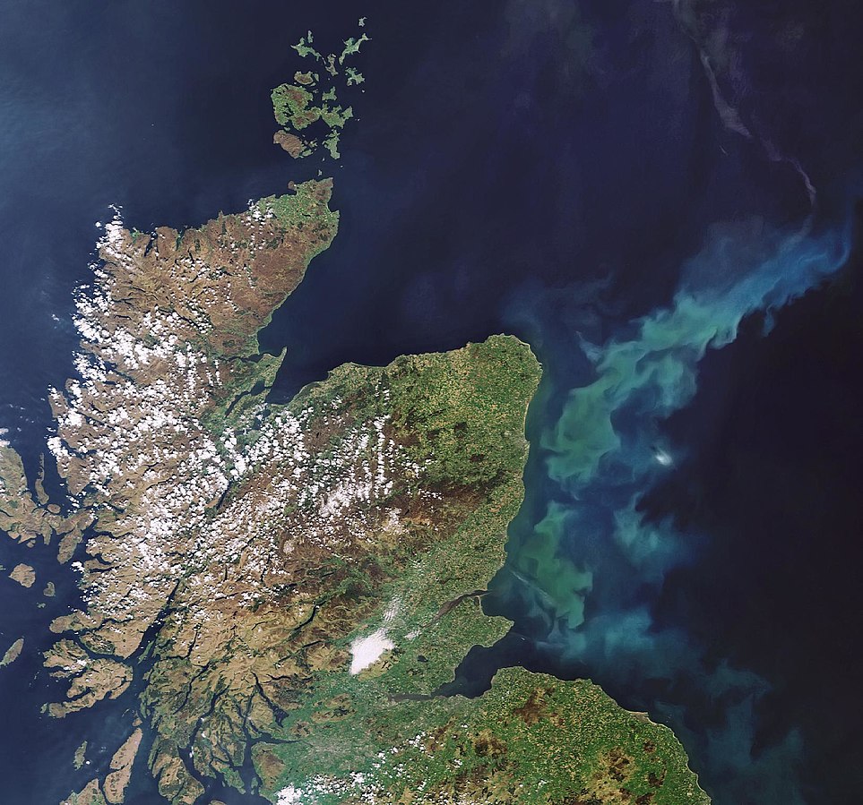
Fig. 7.16 A bloom of phytoplankton off the East coast of Scotland. Image from Envisat via Wikimedia Commons.

Nutrients

To consider the limiting effect of nutrients, we must consider a slightly more complete (but still very approximate) definition of organic matter than (7.17):

(7.18)\[\mathrm{\underbrace{106 CO_2}_{carbon~dioxide} + \underbrace{16 NO_3 + H_3PO_4}_{nutrients} + 78 H_2O + 18H^+ \xrightarrow[+light]{photosynthesis} \underbrace{C_{106}H_{175}O_{42}N_{16}P}_{organic~matter} + \underbrace{150 O_2}_{oxygen}}\]

Here, we include the macronutrients nitrogen and phosphorous alongside carbon, which are two of the main limiting nutrients in the ocean. Also notice that the act of photosynthesis consumes some H⁺, which is involved in the process of nutrient assimilation. An interesting characteristic of organic matter is that it contains C:N:P in a relatively consistent 106:16:1 ratio, which is known as the Redfield Ratio (Fig. 7.17).

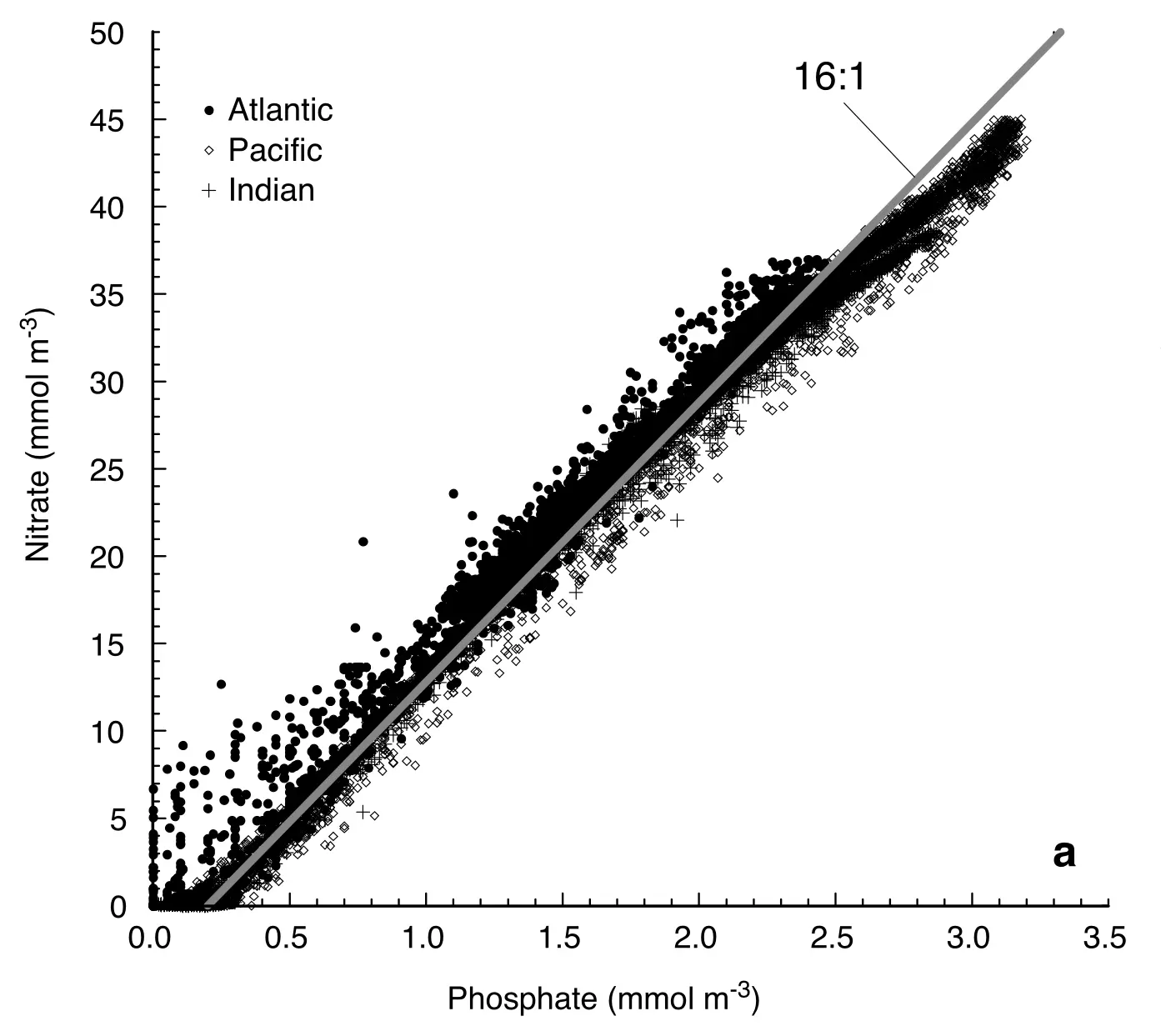
Fig. 7.17 The dissolved concentations of N and P in the ocean show a consistent 16:1 slope, corresponding to the concentration of these elements in average organic matter.

Nutrients will be consumed in proportion to their abundance in organic matter (Fig. 7.18) wherever there is light available to power photosynthesis. This means that, with the exception for the polar oceans where light can be limiting, the patterns of primary productivity are determined by nutrient supply. The mechanisms that supply N and P to the ocean are very different.

Phosphate (PO₄) is derived from the dissolution of rocks on the continents. Consequently, it is either supplied by rivers, or by wind-blown dust, primarily from deserts (dust from the Sahara is regularly found in Central America!).

Nitrate (NO₃) is also supplied from terrestrial sources, but the atmosphere provides a second significant source. Nitrogen is the most abundant element in the atmosphere, which is 78% N₂, but this form of nitrogen is not available for use by phytoplankton. Specialised groups of phytoplankton have evolved the ability to reduce dissolved N₂ into forms that can be used by other phytoplankton, in a process known as nitrogen fixation.

A third source of both N and P to the surface ocean is the upwelling of nutrient-rich deep water, which recycles nutrients from the deep ocean back to the surface. We’ll discuss why the deep ocean is enriched in nutrients below.

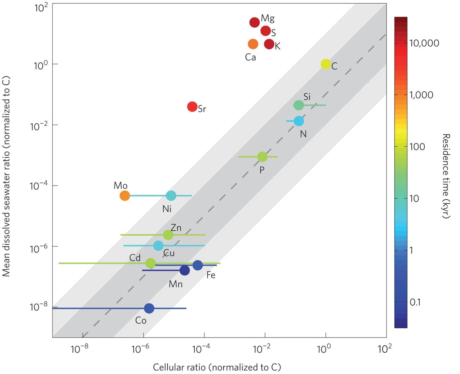
Fig. 7.18 The average concentration of elements in phytoplankton cells and dissolved in the ocean. Anything that falls below the dotted line will limit phytoplankton growth. Consequently, elements below this line (e.g. Fe, Mn, Co) are rapidly consumed by phytoplankton, which gives the ma very short residence time in the ocean compared to abundant ions that are not limiting (e.g. Mg, K, S). From Moore et al. (2013).

Micronutrients…

It is worth noting that N and P are not the only nutrients that limit phytoplankton growth (Fig. 7.18). There are large areas of the ocean where they are abundant, but micronutrients such as iron, manganese, and cobalt, prevent phytoplankton from growing. These patterns of limitation are largely a product of the patterns of the supply of micronutrients on the planet.

The Southern Ocean, for example, is relatively rich in N and P, but has low phytoplankton productivity compared to the Northern hemisphere. This is predominantly driven by low iron concentrations in the Southern Ocean. Iron is low because, like P, it is derived from the dissolution of rocks on the continents, but the antarctic circumpolar current has minimal contact with coastlines that can supply dissolved iron from rivers, and there are no desert regions in the path of the westerlies that blow towards antarctica to supply dust.

The patterns of micronutrient limitation are complex, and beyond the scope of this course. Here, we’ll only consider the effects of macronutrients on phytoplankton growth.

Light

The availability of light for phytoplankton living in the surface is ocean is determined by three main factors:

• Latitude and season, which determine the amount of incident radiation (Fig. 7.19).

• The attenuation of light in the water, which determines how deep light can penetrate into the ocean. This is set by a combination of water depth and turbidity.

• Mixed layer depth, which determines the depth range over which the phytoplankton are living, and the average amount of light they receive.

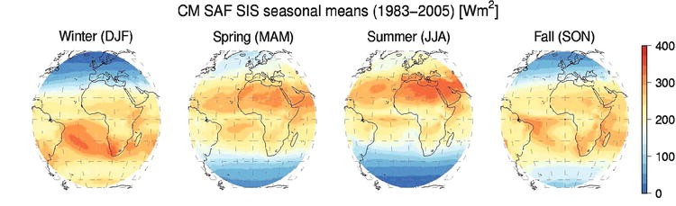
Fig. 7.19 The change in seasonal light availability with season. The high latitudes receive much less light than the low latitudes, and experience several months of near-complete darkness in the winter. From Mueller (2016).

For a phytoplankton to survive it must live, on average, above the compensation depth (Fig. 7.20). The compensation depth is the depth at which the rate of photosynthesis is equal to the rate of respiration. Above this depth, the photosynthesis of the organism exceeds its respiration, and it can grow and reproduce.

Phytoplankton have minimal control over their position in the water column, so are transported throughout the mixed layer by turbulent mixing processes. This means that the average amount of light an individual phytoplankton will receive is determine by a combination of the amount of incident light, the attenuation of light in the water, and the depth of the mixed layer.

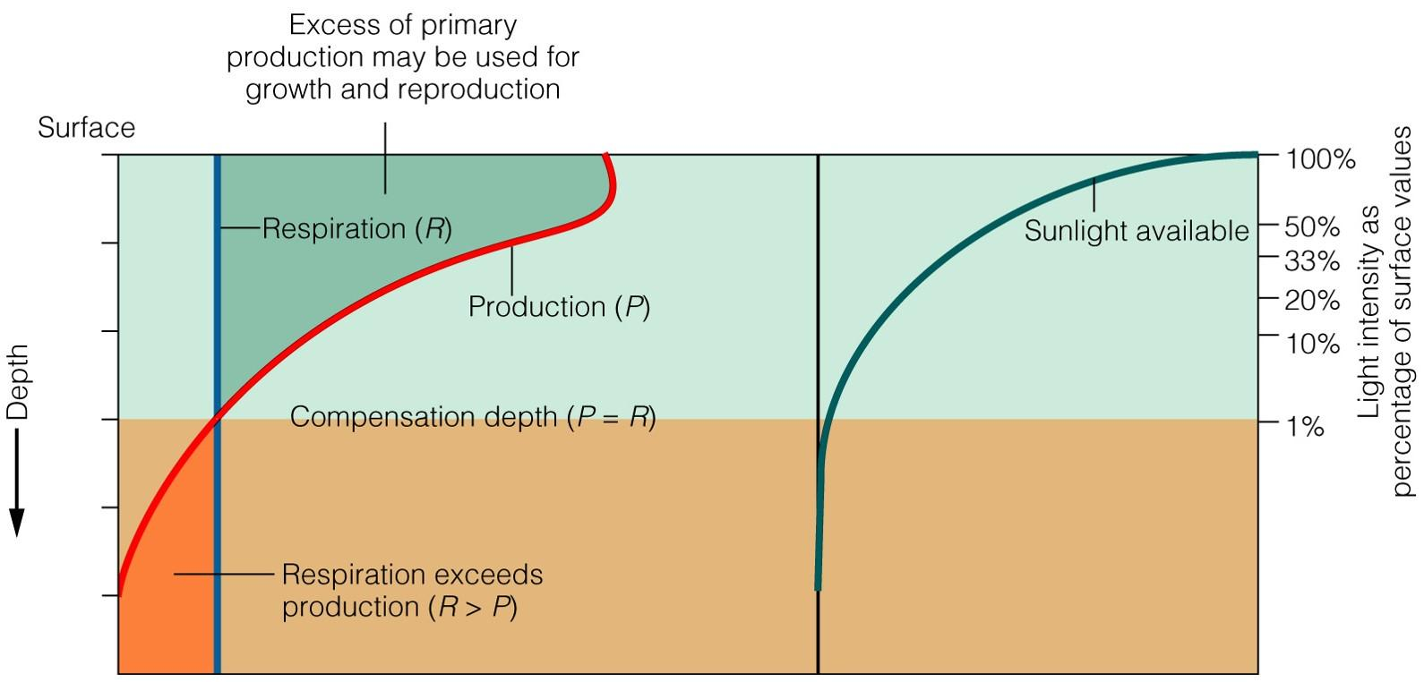
Fig. 7.20 The concept of compensation depth. To grow and reproduce phytoplankton must exist, on average, above the compensation depth in the region where photosynthesis exceeds respiration.

These factors combine to exacerbate the effects of latitude and season on phytoplankton growth. In the high latitudes, winter combines low light levels with a deep mixed layer, which keeps phytoplankton below the compensation depth for much of the year. This allows nutrients to accumulate in the ocean surface, which are then rapidly consumed by phytoplankton when light returns and the mixed layer shallows in the winter. This phenomenon is known as the spring bloom, and is a major driver of primary productivity in the high latitudes. Despite this annual burst of productivity, cold temperatures combined with the months of low light in the high latitudes make them, on average, less productive than the low latitudes, where upwelling of nutrient-rich deep water, readily available light and a relatively shallow mixed layer combine to drive year-round high productivity.

For our purposes, this means that the export of nutrients from the high latitude oceans is less efficient, resulting in a longer residence time of nutrients in the high latitude surface ocean.

The Biological Pump

The Biological Pump describes the transport of nutrients and carbon from the surface ocean to the deep ocean by sinking organic matter (Fig. 7.21). This process is driven by the production of organic matter in the surface waters, which is broken down by bacteria and other organisms as it sinks through the ocean interior, remineralising the organic matter back into its dissolved constituents. This increases the dissolved concentrations of carbon and nutrients in the deep ocean, which are then eventually returned to the surface by Thermohaline Circulation. Broadly speaking, ocean mixing processes try to homogenise the ocean and raise nutrients and carbon to the surface, while the biological pump tries to concentrate nutrients and carbon in the deep ocean. The balance between these processes has a big effect on how much CO₂ is in the atmosphere.

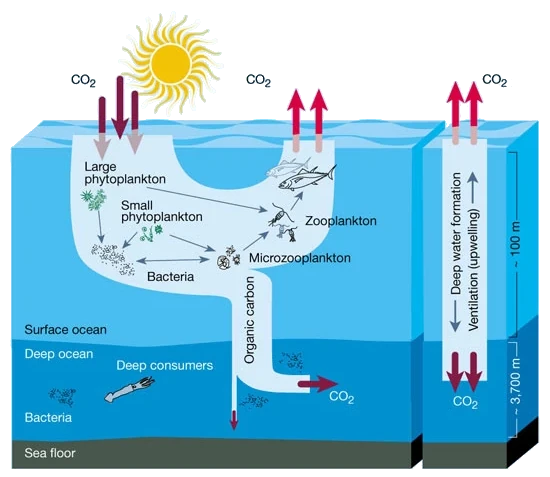
Fig. 7.21 A schematic of the biological pump and solubility pump from Chisholm (2000)

The process of organic matter breakdown is very efficient. Only ~20% of the organic matter produced in the surface ocean makes it into the deep ocean; ~80% is broken down while it is sinking through the surface layer. Only about 1% of the organic matter produced at the surface eventually makes it all the way to the sediments at the bottom of the ocean (but note that sediments are not included in our model, where we assume everything that leaves the surface ocean is remineralised into the deep).

Even though only ~20% of organic matter is exported into the deep ocean, the biological pump is large enough to drive a significant accumulation of nutrients and carbon in the deep ocean, which increases in concentration along the thermohaline circulation path (Fig. 7.22).

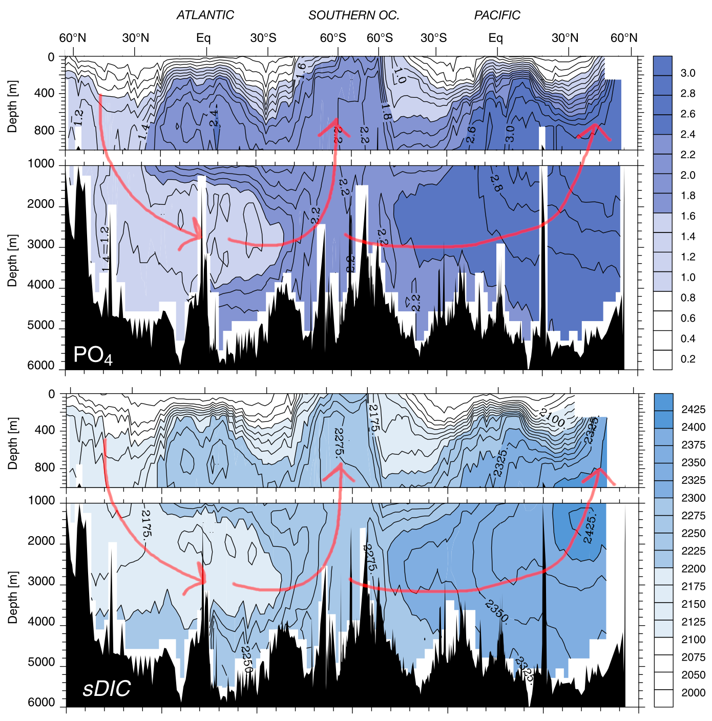
Fig. 7.22 The (salinity-normalised) concentrations of PO₄ and DIC in the ocean interior along the Thermohaline Circulation path (red arrows). Notice how both PO₄ and DIC increase in deep water along the circulation path. This is because they receive a constant supply of nutrients from organic matter falling from the surface and remineralising in the deep water. This acts to concentration nutrients and DIC in the deep ocean, leading to nutrient-rich waters in upwelling zones. From Sarmiento & Gruber (2006), Chapter 5.

The influence of the biological pump can be estimated by subtracting measured DIC concentrations in the deep ocean from patterns predicted by The Solubility Pump alone.

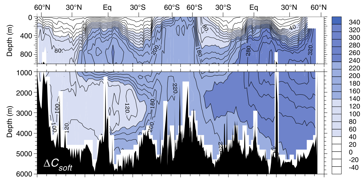
Fig. 7.23 The contribution of the biological pump to the deep ocean carbon reservoir. Sarmiento & Gruber (2006), Chapter 5.

Patterns of Export

Productivity is essential for organic matter export, but is not the only factor that determines how much organic matter is exported from the surface ocean to the deep. The efficiency of the biological pump is governed by the fine detail of the particle characteristics sinking from the surface ocean. Broadly speaking, the rates of remineralisation by bacteria depend primarily on temperature. Therefore, the change of a sinking particle reaching the deep ocean at a given temperature is determined by how long it takes to get there (sinking velocity), and how much of it is left when it does (initial size). This means that, for a set remineralisation rate, larger denser particles will carry more organic matter to the deep ocean than smaller, less dense particles.

The properties of sinking particles, including size, shape and density, are a complex function of the ecosystem living in the overlying water. A particularly efficient way to export organic matter is in the faecal pellets of larger animals, which pre-aggregate organic matter in a single large particle. This can increase the importance of higher trophic levels in driving organic matter export, and make it difficult to relate biological productivity to export efficiency.

Modelling the Biological Pump

To include the biological pump in our model we must:

1. Include a nutrient to limit biological productivity

2. Parameterise the impact of photosynethsis and remineralisation on ocean carbon.

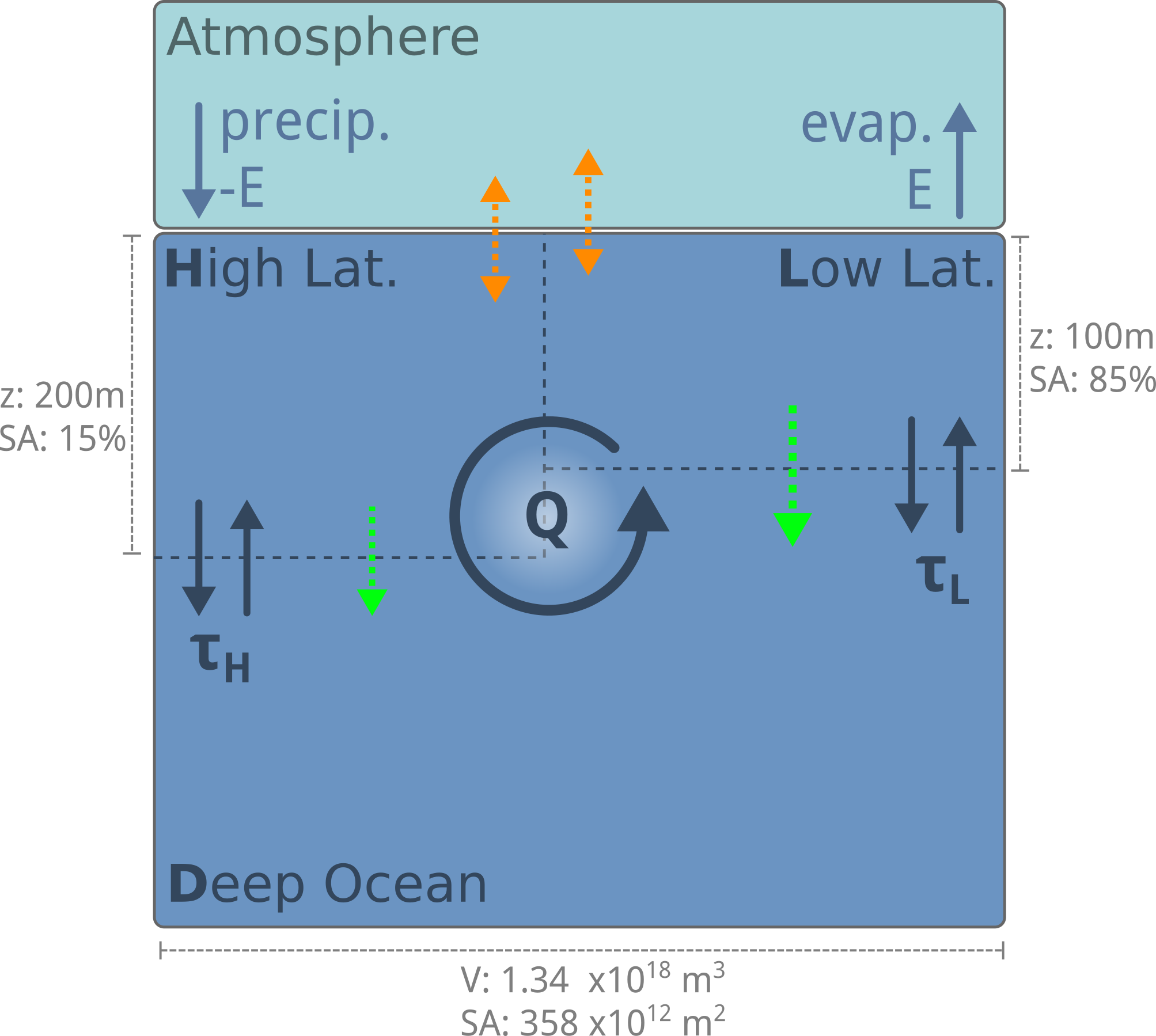
Fig. 7.24 To model the solubility pump, we need to include the conservative transport of a nutrient through the ocean boxes to fuel biological productivity. We then need to paramterise the production of organic matter in the surface ocean, which takes up DIC and nutrients and exports them to the deep ocean.

Adding a nutrient

For our model we will use Phosphate (PO₄) as our limiting nutrient. The choice of P here is arbitrary - you could just as easily use Nitrate, or some other limiting nutrient.

We model phosphate as a conservative tracer that is transported, consumed by phytoplankton in the surface, and released at depth by remineralisation (assuming that everything that leaves the surface box is remineralised in the deep box). As with atmospheric CO₂ exchange, we will model the consumption of P by phytoplankton using a characteristic timescale, \(\tau^P\) (Fig. 7.6). This modifies Eq. (7.2) to:

(7.19)\[\begin{split}\mathrm{\dv{P_L}{t}} &= \mathrm{[\mathrm{transport}] - \frac{1}{\tau^P_L} P_L} \\ \mathrm{\dv{P_H}{t}} &= \mathrm{[\mathrm{transport}] - \frac{1}{\tau^P_H} P_H} \\ \mathrm{\dv{P_D}{t}} &= \mathrm{[\mathrm{transport}] + \left. \left( \frac{V_L}{\tau^P_L} P_L + \frac{V_L}{\tau^P_H} P_H \right) \middle/ V_D \right.} \\\end{split}\]

Where \([\mathrm{transport}]\) represents the thermohaline and vertical mixing terms from (7.2).

Coupling productivity and Carbon

To couple productivity to carbon, we need to relate it to the DIC and TA terms we have already included in our model. To do this, we can write a simplified version of (7.18) that only includes the terms that affect DIC and TA:

(7.20)\[\mathrm{P + 106 DIC - 18 TA \xrightleftharpoons[remineralisation]{photosynthesis} [organic~matter]}\]

Where the relationship with TA is negative because photosynthesis consumes H⁺, which is a negative term in our definition of TA (7.15).

We can therefore link DIC and TA to PO4 via the Redfield Ratio as:

(7.21)\[\begin{split}\mathrm{\frac{d[DIC]_{bio}}{dt}} &= \mathrm{106 \frac{dP_{bio}}{dt}} \\ \mathrm{\frac{d[TA]_{bio}}{dt}} &= \mathrm{-18 \frac{dP_{bio}}{dt}}\end{split}\]

which allows us to include additional biological pumping terms to our DIC expression (7.16) to represent the updtake of DIC in the surface and release at depth:

(7.22)\[\begin{split}\mathrm{\dv{DIC_L}{t}} &= \mathrm{\begin{bmatrix} \mathrm{transport} \\ \mathrm{CO_2~exch.}\end{bmatrix} - 106 \frac{1}{\tau^P_L} P_L} \\ \mathrm{\dv{DIC_H}{t}} &= \mathrm{\begin{bmatrix} \mathrm{transport} \\ \mathrm{CO_2~exch.}\end{bmatrix} - 106 \frac{1}{\tau^P_H} P_H} \\ \mathrm{\dv{DIC_D}{t}} &= \mathrm{[\mathrm{transport}] + \left. \left( 106 \frac{V_L}{\tau^P_L} P_L + 106 \frac{V_H}{\tau^P_H} P_H \right) \middle / V_D \right.}\end{split}\]

and, for TA:

(7.23)\[\begin{split}\mathrm{\dv{TA_L}{t}} &= \mathrm{[\mathrm{transport}] + 18 \frac{1}{\tau^P_L} P_L} \\ \mathrm{\dv{TA_H}{t}} &= \mathrm{[\mathrm{transport}] + 18 \frac{1}{\tau^P_H} P_H} \\ \mathrm{\dv{TA_D}{t}} &= \mathrm{[\mathrm{transport}] - \left. \left( 18 \frac{V_L}{\tau^P_L} P_L + 18 \frac{V_H}{\tau^P_H} P_H \right) \middle / V_D \right.}\end{split}\]

Where the terms in squre brackets represent the conservative transport (7.2) and gas exchange (7.16) terms.

The biological pump is now included in our model, and we can run it to see how it affects the ocean carbon cycle.