Air pollution

5.2. Air pollution#

Sources, sinks and trends

Aims:

To survey the main constituents of air pollution around the world and over time.

To outline the main sources and sinks of different air pollutants, focusing on ${NO}_{2}$ and particulate matter.

To review historic trends of air pollutants and how they are measured.

To apply the Beer-Lambert law to determine the abundance of air pollutants using remote measurement techniques.

Key Points:

Air pollution is not a new phenomenon and work to legislate air pollution can be traced back to the middle ages.

The main air pollutants are oxidising gases ( ${NO}_{2}$ , $O_{3}$ ) and particulate matter.

${NO}_{2}$ is only produced naturally from lightning, it’s main source is the internal combustion engine.

${NO}_{2}$ has a weak chemical-bond which allows low energy photons from the sun to break it apart.

Since the industrial revolution the amount of ${NO}_{2}$ has increased dramatically and disproportionately.

COVID lockdowns showed that ${NO}_{2}$ can be controlled very quickly.

What is air pollution#

Air pollution is a phrase used to describe the presence of contaminants in the air that are harmful for life, to buildings or to climate.

There are lots of different air pollutants. Most are present at trace levels (c.f. the majority of the atmosphere is made up of $N_{2}$ , $O_{2}$ , $Ar$ , and $H_{2} O$ ). These pollutants can come from a range of different sources including, man-made (anthropogenic) and natural – or biogenic.

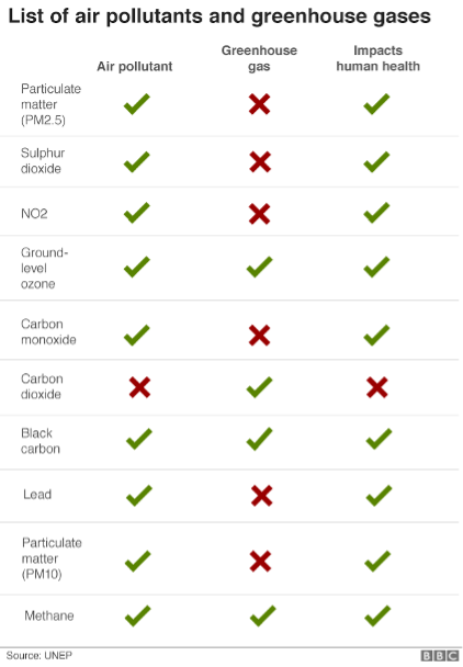
../_images/figure20.1.png — Fig. 5.7 A list many important air pollutants.#

Sources of ${NO}_{2}$ #

The oxides of nitrogen ( ${NO}_{x} = NO + {NO}_{2}$ ) play a dominant role in the chemistry of the troposphere, as we will find in the following sections. They arise from a combination of natural and anthropogenic sources. Road transport is an important and rapidly growing ${NO}_{x}$ source. Most lightning is associated with deep convection and the largest sources are in the tropics. Only lightning and aircraft are non-surface sources.

Table 5.2 Sources (and ranges of uncertainty) of atmospheric ${NO}_{2}$ .#
Sources	${TgNO}_{2} {yr}^{- 1}$
Fossil fuel combustion	$20 (14 - 28)$
Release from soils	$20 (4 - 40)$
Biomass burning	$12 (2 - 24)$
Lightning discharges	$8 (2 - 20)$
${NH}_{3}$ oxidation	$3 (0 - 10)$
Ocean surface	$< 1$
Aviation	$0.5$
Injection from the stratosphere	$0.1 (0.6$ total ${NO}_{y})$
Total sources	$64 (25 - 112)$

Table 5.3 Sinks (and ranges of uncertainty) of atmospheric ${NO}_{2}$ .#
Sinks	${TgNO}_{2} {yr}^{- 1}$
Wet decomposition of nitrate (land)	$18 (8 - 30)$
Wet deposition of nitrate (ocean)	$8 (4 - 12)$
Dry deposition of ${NO}_{x}$	$16 (12 - 22)$
Total sinks	$43 (24 - 64)$

${NO}_{2}$ absorbs strongly in the UV and visible part of the solar spectrum. This has two important consequences.

${NO}_{2}$ undergoes photolysis (photodissociation) rapidly.
${NO}_{2}$ can be observed easily from space.

Making use of point 2 above, the figure below shows maps of the distribution of ${NO}_{2}$ .

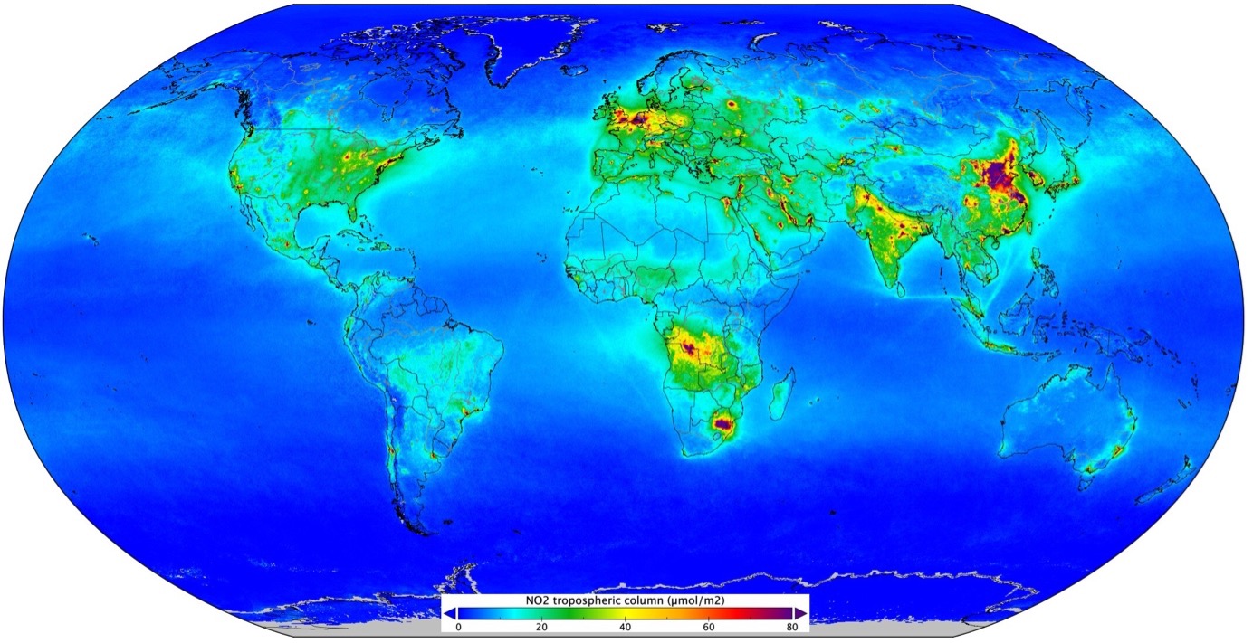
../_images/figure20.3.jpg — Fig. 5.8 Measurements from the Copernicus Sentinel-5P satellite mission between April and September 2018. Credit ESA and KNMI.#

Photodissociation#

The photo-reaction: $AB + h v = A + B$

Has an associated rate constant (or photolysis frequency) $J_{AB} / s^{- 1}$ and a rate of reaction $R_{J} / molecules {cm}^{- 3} s^{- 1}$ , where $R_{J} = J_{AB} \times [AB]$

The rates of change of the molecules are:

(5.11)#

\frac{d [AB]}{d t} = - \frac{d [A]}{d t} = - \frac{d [B]}{d t} = - J_{AB} [AB]

Calculation of photolysis frequency $J$ #

The photolysis frequency $J_{i}$ of constituent $i$ is defines as:

(5.12)#

J_{i} = \int_{λ = 0}^{\infty} I_{λ} σ_{λ, i} ϕ_{λ, i} d λ

where $σ_{λ, i}$ is the wavelength dependent absorption cross-section $({cm}^{2})$ , $ϕ_{λ, i}$ is the wavelength dependent quantum yield (efficiency), and $I_{λ}$ is the photon intensity at wavelength $λ$ .

To calculate the photon intensity with the atmosphere at altitude $z$ , it is necessary to compute the transmission of the atmosphere at that wavelength. To do this we use the Beer Lambert Law:

(5.13)#

I_{λ, z} = I_{λ, \infty} e^{- D_{λ}}

where $I_{λ, \infty}$ is the photon intensity at the top of the atmosphere, and $D_{λ}$ is the atmospheric optical depth, defined as:

(5.14)#

D_{λ} = \sum_{i} σ_{λ, i} N_{i}

where the summation is over all $i$ absorbing species, $σ_{λ, i}$ is the cross-section $({cm}^{2})$ , and $N_{i}$ the total number of molecules of absorbing species $i$ between $z$ and the top of the atmosphere ( ${cm}^{- 2}$ ).

To an excellent approximation we need only to consider $O_{2}$ and $O_{3}$ when calculating the $D_{λ}$

In each case $N$ is defined as:

(5.15)#

N = \int_{z}^{\infty} {[n]}_{z} d z

where ${[n]}_{z}$ is the concentration of $O_{2}$ or $O_{3}$ at altitude $z$ .

Calculation of $N_{O_{2}}$ is straightforward as $O_{2}$ is uniformly mixed in the atmosphere.

The major factors determining fluxes of radiation in the visible and UV wavelengths in the atmosphere are absorptions by $O_{2}$ and $O_{3}$ . Other factors include Rayleigh scattering, and in the troposphere, the presence of clouds which can act to increase or reduce photolysis rates, and the Earth’s albedo.

Figure 5.2 shows the regions of the spectrum where the bands of $O_{2}$ and $O_{3}$ which absorb in the Earth’s atmosphere are located ( $O_{3}$ has an additional weakly absorbing band at visible wavelengths – the Chappuis band).

A detailed knowledge of the absorption properties of the atmosphere is required for a full understanding or for accurate modelling of atmospheric photochemistry. However, there are a number of wavelengths which are of particular significance for understanding some of the basic principles. Firstly, $λ = 242 nm$ is the longest wavelength (i.e. the lowest energy) at which photons can dissociate $O_{2}$ thereby producing $O_{3}$ directly from $O_{2}$ :

O_{2} + h ν \to O + O

O + O_{2} + M \to O_{3} + M^{*}

Secondly $λ =\sim 400 nm$ is the longest wavelength at which ${NO}_{2}$ can be photolysed ( ${NO}_{2}$ does absorb at longer wavelengths, but the quantum yield for dissociation falls rapidly to zero). The fate of the ground state $O$ atom formed is to recombine with $O_{2}$ thereby indirectly forming $O_{3}$ :

{NO}_{2} + h ν \to NO + O

O + O_{2} + M \to O_{3} + M

Also, $λ =\sim 310 nm$ is also highly significant as it is the longest wavelength at which $O_{3}$ can be photolysed to form excited atomic oxygen $O (^{1} D)$ , leading to the production of $OH$

Changes in ${NO}_{2}$ over time.#

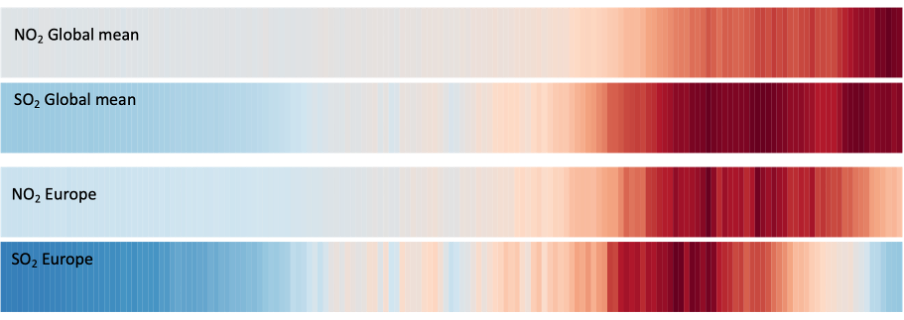
../_images/figure20.4.png — Fig. 5.9 Modelled changes in ${NO}_{2}$ and ${SO}_{2}$ from 1850 to 2014 highlight the rise (and decline) of these pollutants across the globe (and Europe).#

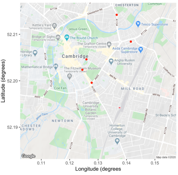
../_images/figure20.5.png — Fig. 5.10 A map of cambridge with monitoring stations shown.#

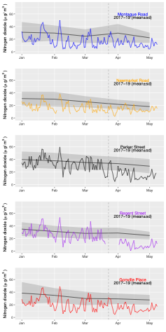
../_images/figure20.6.png — Fig. 5.11 The impacts of the COVID lockdowns on ${NO}_{2}$ levels across Cambridge at the locations shown in Fig. 5.10. The clearest signal of change is at Regent Street and Parker Street, where levels dropped to unprecedentedly low levels.#

Air pollution

Contents

5.2. Air pollution#

What is air pollution#

Sources of NO2#

Photodissociation#

Calculation of photolysis frequency J#

Changes in NO2 over time.#

Sources of ${NO}_{2}$ #

Calculation of photolysis frequency $J$ #

Changes in ${NO}_{2}$ over time.#