How much carbon is in the ocean?

7.1. How much carbon is in the ocean?#

Tracers in the sea: Ocean movement and biogeochemistry.

Key Points:

There is ~50x more carbon in the ocean than in the atmosphere.

The ocean is the largest reservoir of ‘available’ carbon on Earth’s surface.

Carbon in the ocean is heterogenerously distributed.

Ocean circulation, chemistry and biology interact to drive a disequilibrium between the atmosphere and average ocean composition.

A model must have at least 3 boxes to simulate these processes.

Why are the oceans important for carbon?#

The oceans are large - they cover ~71% of the Earth’s surface, with an average depth of 3.7 km. They are also dense, with a total mass of 1.4 x10²¹ kg. This is around 300 times more massive than the atmosphere (5.148 x10¹⁸ kg). The oceans also contain a lot that isn’t water.

The sheer size and density of the oceans makes it a globally-important reservoir of dissolved chemicals, even if they are only present at low concentrations. The most immediate example of this is salt. Each kg of seawater contains ~35 g of dissolved solids, which represents the long-term balance of rock weathering and formation on Earth’s surface.

The ocean is also a significant store of dissolved carbon. Gasses exchange between the ocean at the atmosphere, which allow it to store dissolved CO₂. The movement of these dissolved gasses around the ocean can have a major impact on atmospheric composition, and particularly CO₂ concentration.

How much carbon is in the ocean?#

Oceanographers have taken a lot of measurements of carbon dissolved in the ocean. These measurements show that the concentration of Dissolved Inorganic Carbon (DIC) varies widely, with an average 2255 μmol kg^-1. Combined with the mass of the ocean (~1.4x10²¹ kg), we can calculate that there are ~37,900 PgC dissolved in seawater (Fig. 7.1). This is around 50x more than is present in the atmosphere today (~750 GtC).

Calculation…

\[\begin{split} \begin{align*} 2255 ~\mathrm{μmol~C~kg^{-1}} \times 10^{-6} &= 0.002255 ~\mathrm{mol~C~kg^{-1}} \\ 0.002255 \times 12 ~\mathrm{g~mol^{-1}} &= 0.02706 ~\mathrm{g~C~kg^{-1}} \\ 0.02706 \times 1.4 \times \mathrm{10^{21}~kg} &= 3.7884 ~\mathrm{\times 10^{19}~g~C} \\ 3.7884 \times 10^{-15} &= 37,884 ~\mathrm{Pg~C} \end{align*} \end{split}\]

where 12 is the atomic mass of carbon.

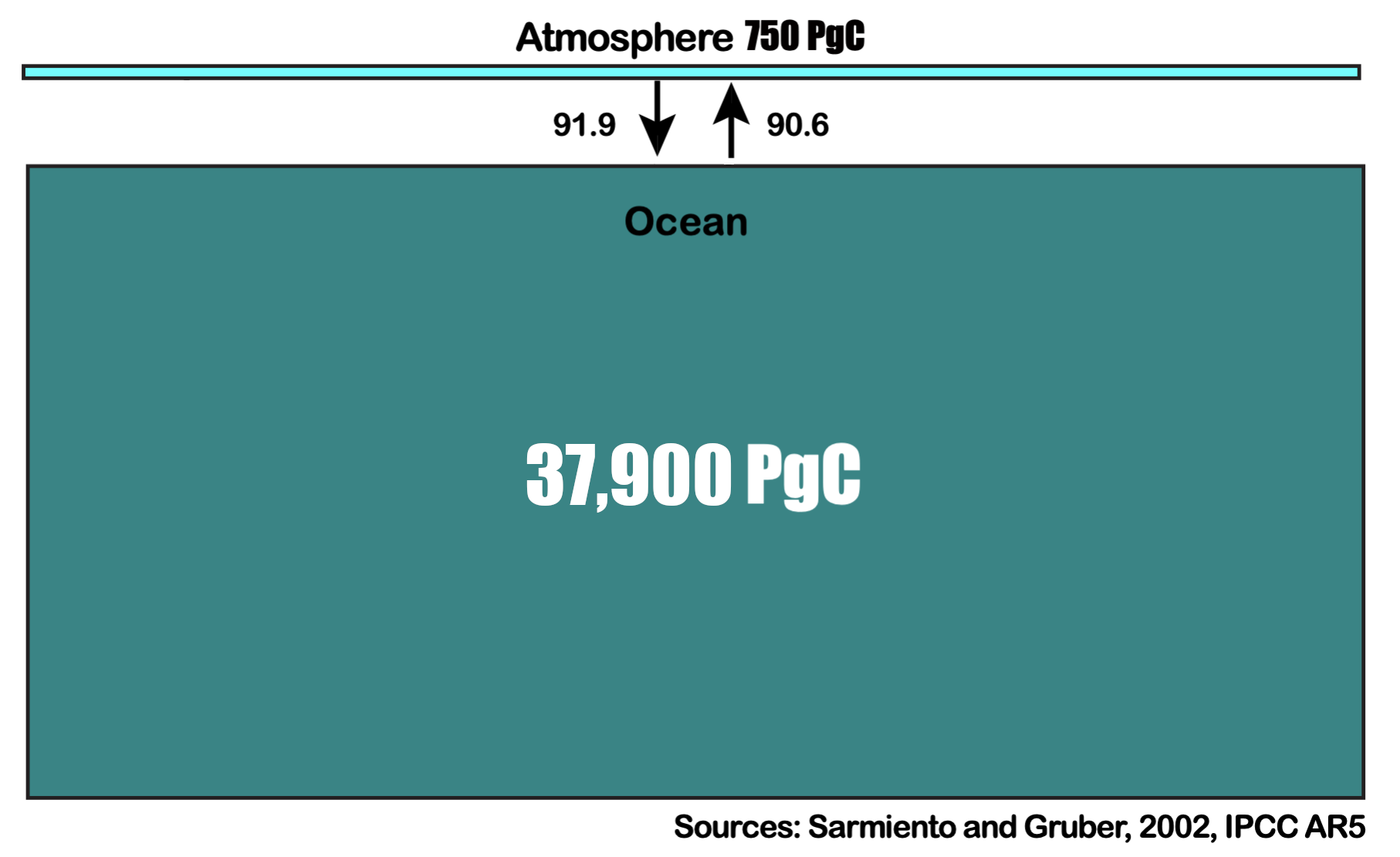
../_images/carbon-1box.png — Fig. 7.1 The amounts of carbon in the ocean and atmosphere and the exchange between them in the modern ocean. The area of each box is proportional to the size of the reservoir.#

Ocean-Atmosphere Exchange#

The exchange of carbon between the ocean and atmosphere is large, with an annual flux of ~90 PgC (Fig. 7.1) - around 12% of the carbon in the atmosphere moves between the ocean and the atmosphere each year. In the modern ocean, there is slightly more uptake than release, making the ocean a net sink for carbon taking up 1.7±0.7 PgC yr^-1. Emissions from fossil fuel burning are currently 7.8±0.6 PgC yr^-1, so the ocean is currently taking up ~20% of the carbon we are releasing. Since the start of the industrial revolution, it is estimated that the ocean has taken up 30-50% of the carbon we have released. The large uncertainties on these numbers reflect the complexity of the processes involved, and the difficulty of measuring them.

Carbon moves between the ocean and atmosphere by the exchange of CO₂ molecules. The exchange of molecules between gas and liquid is described by Henry’s Law, which states that the solubility of an ideal gas in a liquid is proportional to the partial pressure of the gas in the overlying air:

\[C = k P\]

where \(C\) is the concentration of the gas in the liquid, \(k\) is the solubility constant, and \(P\) is the partial pressure of the gas in the atmosphere. For CO₂, we write:

(7.1)#\[[CO_2] = K_0\ pCO_2\]

where \(K_0\) is the solubility constant for CO₂ in water, and \(pCO_2\) is the partial pressure of CO₂ in the atmosphere, and square brackets denote the concentration of a dissolved chemical species.

The value of \(K_0\) depends on temperature and salinity. Temperature has by far the strongest effect, with \(K_0\) decreasing from ~0.07 to ~0.02 between 0-35°C. The influence of salinity is minor, with slightly higher values in fresher water.

For average surface ocean conditions of 20°C and 35 PSU, \(K_0\) has a value of ~0.03. This means that if carbon in the oceans and atmosphere were in equilibrium, the atmosphere would contain 2255 / 0.03 = ~75,200 ppm CO₂!

As of January 2024, the atmosphere contains 422.8 ppm CO₂ (up by 3.3 ppm from last year!).

Equilibrium?#

This back-of-the-envelope calculation shows that the average ocean contains ~175x more carbon than is predicted by a simple 1-box model of ocean-atmosphere exchange. The atmosphere is not in equilibrium with the ‘average’ ocean.

There are three main reasons why the atmosphere appears to be out of equilibrium with the average ocean, which we will examine in detail in the next three lectures:

The ocean has structure - it circulates and is stratified. Only CO₂ in the surface of the ocean can exchange with the atmosphere (Fig. 7.2).
CO₂ reacts with water to form non-gaseous dissolved species. The chemistry of carbon in seawater changes how much CO₂ is available to equilibrate with the atmosphere.
Biological processes in the surface ocean absorb up carbon from the atmosphere and transport it to the deep ocean, where it cannot equilibrate with the atmosphere.

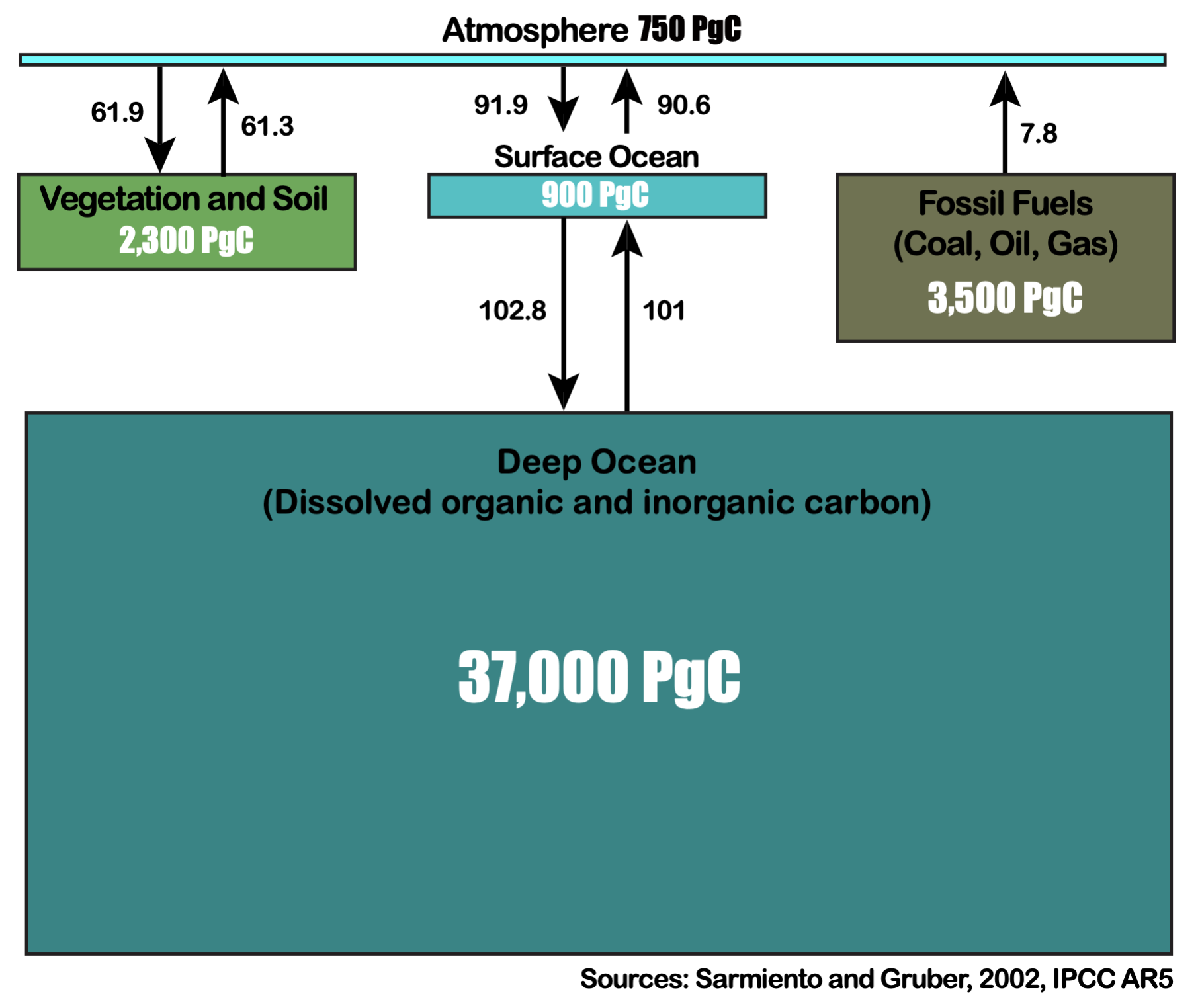
../_images/carbon-components.png — Fig. 7.2 The amount of carbon in each of the main available reservoirs at Earth’s surface, and the fluxes between them. The deep ocean contains by far the largest amount of carbon, so small changes in the processes that partition carbon between the surface and deep ocean can have a major impact on atmospheric CO₂ concentration. In its current configuration, the deep ocean is a net sink of carbon, taking up ~1.8 PgC yr^-1.#

Together, these processes act to move carbon from the surface to the deep ocean where it cannot exchange with the atmosphere. The surface ocean contains a much smaller pool of ~900 PgC, only ~0.5% of which is present as CO₂ that can exchange with the atmosphere.

The oceans are a key component of the global carbon cycle (Fig. 7.3), containing both the largest reservoir of readily available carbon and the largest fluxes to and from the atmosphere. The sheer amount of carbon stored in the deep ocean means that small changes in the processes that transfer carbon from atmosphere to surface ocean, or surface ocean to deep ocean, can have a major impact on atmospheric CO₂ concentration.

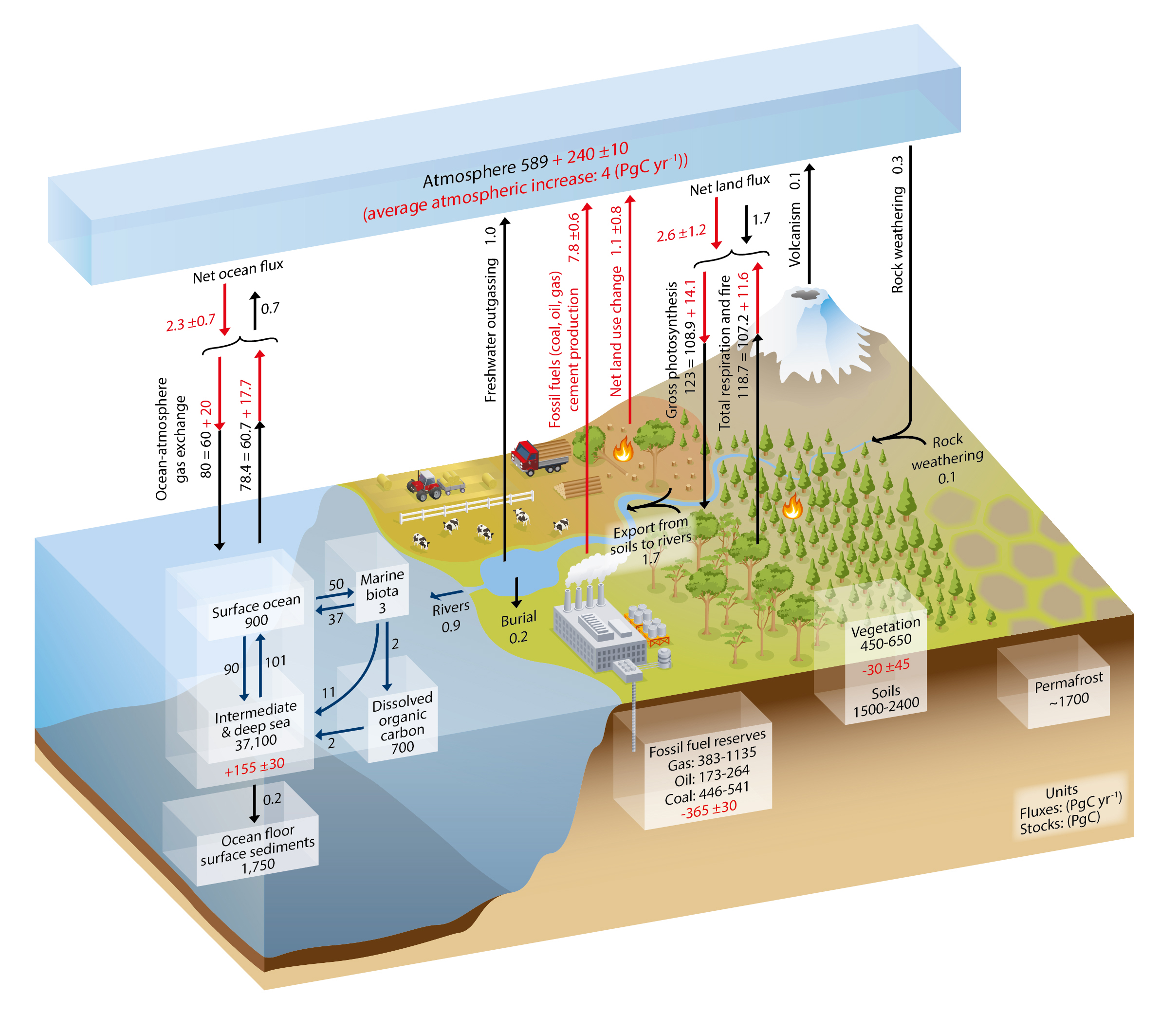
../_images/ipcc-carbon-cycle.jpg — Fig. 7.3 The processes of carbon release and uptake in the modern world. ‘Undisturbed’ fluxes are shown in black, and the influence of human activities is shown in red. From IPCC AR5, Chapter 6.#

From the perspective of understanding climate change, the timescales of these storage and release processes are critical. You will recall from the Global Environment lectures that the timescales of normal ocean circulation are relatively slow (100s-1000s of years), so you might expect that the timescales of carbon storage and release in the ocean to be similar. However, as you saw in the Stommel box model for ocean heat transport, switching between multiple stable circulation states can be much more rapid, bringing associated changes in the uptake and release of carbon from the ocean. Biological processes in the surface ocean can also react much faster than circulation changes (10s-100s of years), making all these processes critical in predicting how the uptake and release of carbon from the ocean will change in the future.

Modelling Ocean Carbon#

In the coming lectures and practicals we will construct a model of the carbon cycle in the ocean. This model has some similarities to the Stommel Model of ocean circulation, with global thermohaline circulation driven by density gradients between the low and high latitudes. However, to model ocean carbon we must be able to represent the vertical stratitification of the ocean that physically separates carbon in the surface ocean that can exchange with the atmosphere from carbon in the deep ocean which cannot.

We simulate this stratification by restricting the high- and low-latitude boxes you used in the Stommel model to representing the surface ocean, and adding a deep ocean reservoir underlying both these boxes. This provides the necessary latidudinal structure to represent ocean circulation, and the vertical structure to represent the ocean carbon cycle. We will also add an overlying atmosphere to the model, which will allow us to represent the exchange of carbon between the ocean and atmosphere.

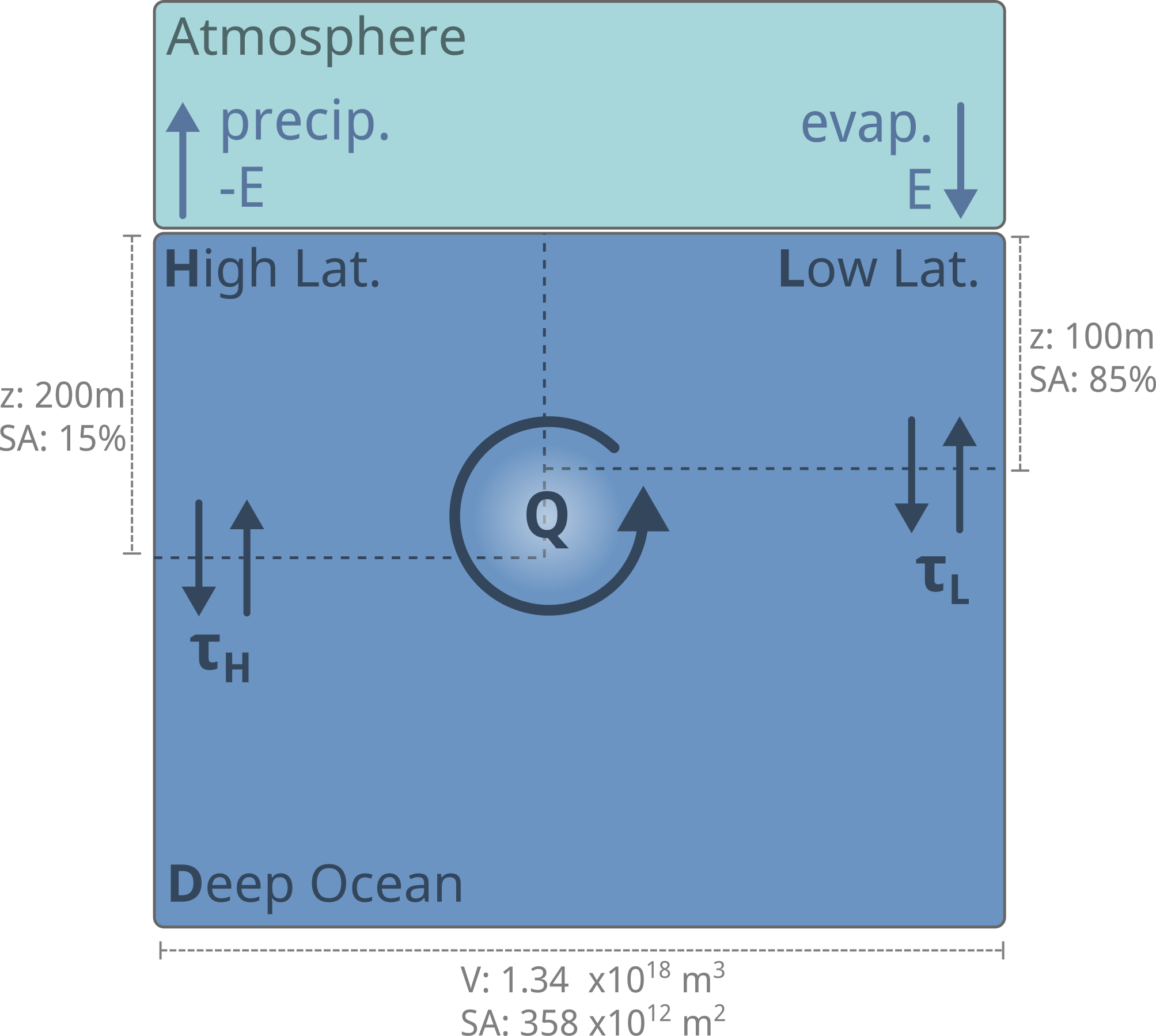
../_images/ocean-3box.png — Fig. 7.4 The geometry of our model of the ocean carbon cycle containing 3 ocean boxes and an overlying atmosphere box. For the purposes of carbon, the atmosphere is considered as a well-mixed reservoir. This is a reasonable approximation because atmospheric transport is so much faster than ocean circulation. Q represents the thermohaline circulation (THC) flux, E is the change in salinity due to evaporation, and τ represents the timescale of mixing at the base of the surface boxes, which can be considered as a diffusion process.#

Boxes to Reality#

To understand why we’re dividing the ocean this way, let’s take a look at the temperature structure of the ocean (Fig. 7.5). You can see the broad-scale transport structure we’re trying to represent in the downwelling and upwelling of water at high and low latitudes, respectively, along with the tendency for the different boxes to have distinct physical properties (in this case the average temperature of each box, and the depth of the base of the surface boxes).

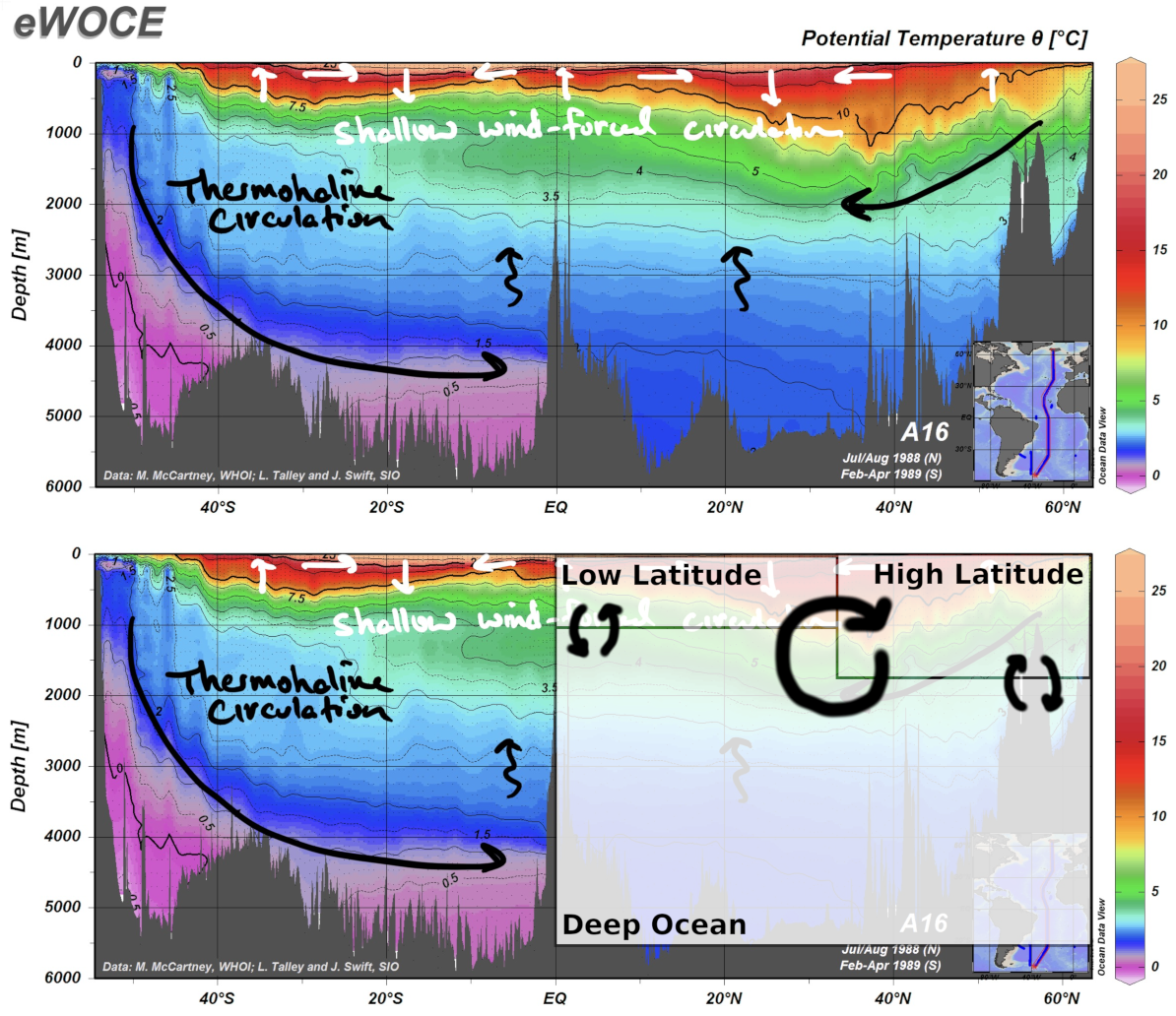
../_images/ocean-circulation-boxes.png — Fig. 7.5 The geometry of our model relative to the real ocean. The THC flux represents the sinking of water at high latitudes and upwelling at low latitudes driven by density gradients, as in the Stommel model. The surface-deep exchange fluxes represents smaller-scale wind-driven mixing between the surface and deep ocean. By comparison to the underlying temperature plot, you can see that these boxes offer a coarse approximation of the ocean structure. To make a more realistic model, you might consider adding more boxes to better represent the vertical and horizontal structure of the ocean.#

Conservative Transport#

To get a feel for how this model works, we will start by writing the equations to describe the transport of a conservative tracer, \(C\), around the model. A conservative tracer is neither created nor destroyed in the model - the total amount in the system remains the same, although model processes can partition it unevenly between the boxes.

To do this, we must account for thermohaline circulation (\(q\)), which creates a directional flux between the three boxes, and surface-deep exchange, which creates bi-directional fluxes between each surface box and the deep box. We represent this surface-deep exchange using a characteristic timescale, \(\tau\), which describes the amount of time it would take for the box to equilibrate with the deep ocean (Fig. 7.6).

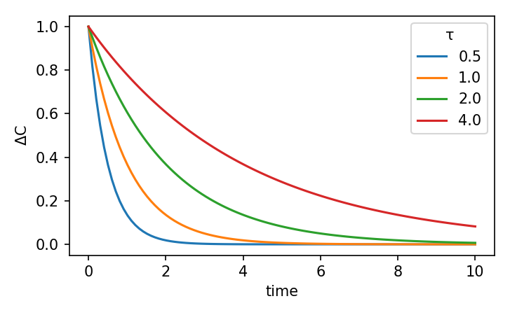
../_images/carbon-tau.png — Fig. 7.6 The effect of different \(\tau\) values on the equilibration time between to reservoirs.#

Together, these two mixing processes give us:

(7.2)#\[\begin{split}\dv{C_L}{t} &= \underbrace{\frac{q}{V_L} (C_D - C_L) - \frac{1}{\tau^{mix}_L} ( C_L - C_D )}_{\mathrm{[transport]_L}} \\ \dv{C_H}{t} &= \underbrace{\frac{q}{V_H} (C_L - C_H) - \frac{1}{\tau^{mix}_H} ( C_H - C_D )}_{\mathrm{[transport]_H}} \\ \dv{C_D}{t} &= \underbrace{\frac{q}{V_D} (C_H - C_D) + \left. \left( \frac{V_L}{\tau^{mix}_L} ( C_L - C_D ) + \frac{V_H}{\tau^{mix}_H} ( C_H - C_D ) \right) \middle/ V_D \right.}_{\mathrm{[transport]_D}}\end{split}\]

Where the subscripts \(L\), \(H\), and \(D\) refer to the high, low, and deep boxes, respectively. These equations are very similar to the Stommel Model, but with the addition of a deep ocean box. In subsequent expressions we will express these as ‘\(\mathrm{[transport]_x}\)’ for simplicity.

Notice a key difference here is that we have to take the volume (\(V\)) of each of the boxes into account when calculating transport of dissolved constituents.

All properties of each box will be influenced by these transport processes, so these equations will apply to all tracers included in our model.

3-box Circulation#

We will drive circulation in our model in the same way as in the Stommel model, where we calculate \(q\) from the density gradient between the \(L\) and \(H\) surface boxes. This density difference is caused by temperature exchange between the ocean and atmosphere and by evaporation modifying the salinity of the water.

(7.3)#\[q_T = k (\alpha \Delta T - \beta \Delta S)\]

where \(\Delta T\) and \(\Delta S\) are the \(L - H\) temperature and salinity gradients, respectively.

To calculate the transport of salinity (\(S\)) we add evaporation and precipitation, \(E\), to (7.2), which adds salt (by evaporation) in the low latitudes and removes salt (by dilution) in the high latitudes, to get:

(7.4)#\[\begin{split}\dv{S_L}{t} &= \mathrm{[transport]_L} + \frac{E}{V_L} \\ \dv{S_H}{t} &= \mathrm{[transport]}_H - \frac{E}{V_H} \\ \dv{S_D}{t} &= \mathrm{[transport]}_D \\\end{split}\]

where \(\mathrm{[transport]}\) represents the conservative transport terms from (7.2).

To calculate the transport of heat (temperature, \(T\)), we add terms for the exchange of heat between the ocean and atmosphere to (7.2) to get:

(7.5)#\[\begin{split}\dv{T_L}{t} &= \mathrm{[transport]}_L - \frac{1}{\tau^{T}_L} (T_L - T_A ) \\ \dv{T_H}{t} &= \mathrm{[transport]}_H - \frac{1}{\tau^{T}_H} (T_H - T_A ) \\ \dv{T_D}{t} &= \mathrm{[transport]}_D \\\end{split}\]

Note that neither \(E\) nor \(\tau^T\) influences the deep box directly because it is not in contact with the atmosphere. Any change in surface properties must therefore be communicated to the deep box through the mixing fluxes, which adds a significant delay to the response time of the deep ocean.

Numerical Solutions#

The addition of a deep box makes it impossible to solve this model analytically. Even if it were possible at this stage, the addition of new, interacting ocean properties in future (carbon and nutrients) would rapidly make the model intractable. We will therefore be solving this model numerically in practicals by running simulations.