7.5. Future Oceans

Key Points:

• The model we have made in this section is a minimal representation of the ocean carbon cycle.

• We have approximated many important processes using characteristic timescale parameters (\(\tau\)).

• These \(\tau\) values are independent of the state of the model, which is not realistic.

• Adding these dependencies allows us to explore the importance of these interactions for the future ocean carbon cycle.

• Here, we look at how you might investigate the impact of ocean acidification in this model.

• You will do something similar for your Lab Report!

A Model Ocean

The model we have put together in the Ocean Carbon section (Fig. 7.32) does a decent job of representing the state of the ocean carbon cycle. Provided with average surface temperatures, evaporation rates, it predicts the partitioning of carbon between the deep ocean, the surface ocean and the atmosphere we see in the modern world based on the chemical and biological processes occurring in the ocean. However, it is a gross over-simplification of the real ocean, with only three boxes and with all the key processes governed by relatively few key parameters (Table 7.1) that are independent of the state of the model.

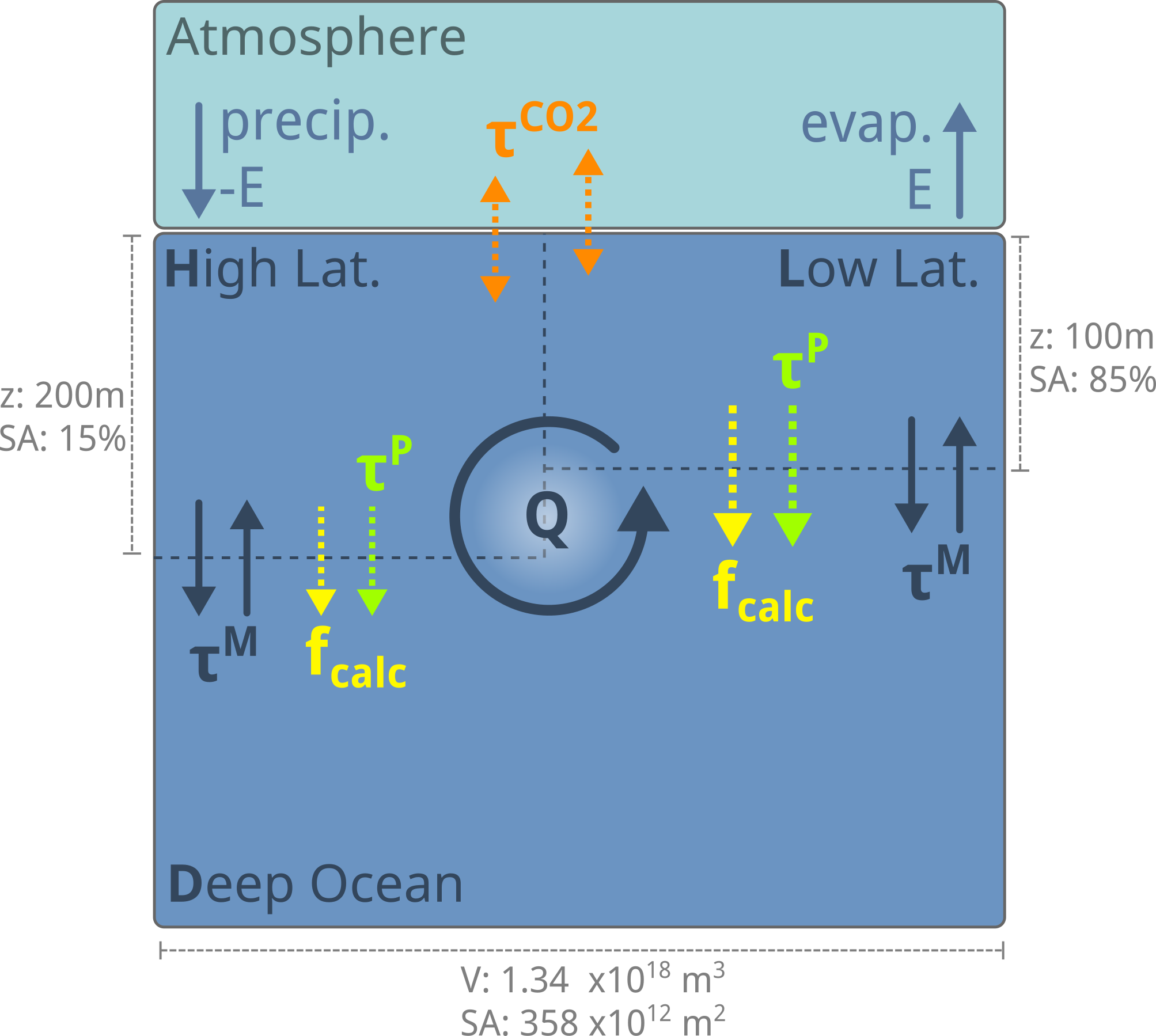
Fig. 7.32 The model of the ocean carbon cycle we have put together in this section, along with the key \(\tau\) parameters that control its behaviour.

As we have seen in our consideration of The Solubility Pump, The Biological Pump and The Carbonate Pump, there are good reasons for the processes behind these simple timescale parameters to interact with each other, and be sensitive to the state of the model (Table 7.1). These sensitivities provide potentially critical positive and negative feedbacks in the modern ocean carbon cycle that might dramatically alter the trajectory of future ocean carbon uptake. If we want to use our model to explore how the ocean might respond to the continued emissions of CO₂, we must include some of these dependencies in our model.

Table 7.1 Model Parameters, the processes they represent, and the factors those processes might depend on.

Parameter	Process	Could be influenced by…
\(\tau^T\)	Surface-Atmosphere temperature exchange	Surface mixing, wind strength, cloud cover
\(E\)	Evaporation-precipitation	Air temperature, wind strength, cloud cover
\(\tau^{M}\)	Surface-deep mixing	Wind strength, mixed layer depth changes, stratification
\(\tau^{CO2}\)	Surface-Atmosphere CO\(_2\) equilibration	Surface mixing rates, wind strength
\(\tau^{P}\)	Organic matter export	Limiting micronutrient, ecosystem structure, light availablity, mixed layer depth, temperature, pH, [CO2], particle sinking charactersitics
Redfield Ratio	Composition of exported organic matter	Ecosystem structure
\(f_{calc}\)	Export of CaCO3 associated with organic matter	Ecosystem structure, saturation state, particle sinking charactersitics

Model Evolution

The process of model development we are following here is very similar to how climate models have evolved in the last few decades. The 3-box model we have made is inspired by a model developed by Sarmiento & Toggweiler in 1984, who used it to propose that observed 70ppm pCO₂ changes observed in ice cores over glacial-interglacial cycles were driven by changes in high-latitude ocean productivity. This simple model was sufficient to consider first-order questions about ‘why did pCO₂ change by 70ppm between the ice ages?’, as it was able to demonstrate the sensitivity of pCO₂ to regime shifts in ocean mixing and productivity.

In the modern world, we are concerned with how the ocean will respond to the anthropogenic release of CO₂ and consequent warming. Global emissions stand at around 8 PgC yr^-1, about 4 PgC yr^-1 of this remains in the atmosphere, and the ocean takes up 2.3±0.7 PgC yr^-1. Small changes in how carbon is partitioned between the ocean and the atmosphere could have a substantial impact on the rate of CO₂ increase in the atmosphere. The three-box model with independent processes that we have developed is too coarse to accurately answer these questions. We need a model that represents the interaction ocean processes and the geographic variability of the ocean in much more detail to precisely tackle these questions.

The need for precision in these estimates has led to the development of increasingly complex climate models, which have evolved by extending the same conceptual approach that we have used to build our simple model. They have simply added more boxes to represent spatial differences in the atmosphere, land and ocean, included more processes that move heat and chemicals around the planet, and parameterised some of the state-dependence of these processes, and the interactions between them.

The end result is a variety of Global Climate Models (GCMs) that are used to simulate the climate of the Earth, and to predict how it will change in the future. Ultimately, these models are still just a set of equations that represent the processes that drive the climate system, and the parameters that control those processes, just like the model we have developed.

Modelling Ocean Acidification

For the rest of this section, we will explore one example of how we might extend our simple model to include the impact of ocean acidification on the export of CaCO₃ from the surface ocean.

Lab Report!

This is similar to the type of exercise you will be asked to complete for the final section of your Lab Report. You will be provided with a few scenarios, which will require you to modify your model to include a new process or interaction, then you will be asked to explore the impact of these scenarios on the model. You will be provided with an example lab report write-up, along with code implementing all of the changes below, with the answers to Practical 15.

Example Questions

…of the type you can expect to be asked for the Lab Report are highlighted below in boxes like this.

Ocean Acidification

Ocean acidification has so far come up in two places: in The Solubility Pump we saw that increasing pCO2 decreases ocean pH, and when discussing The Carbonate Pump we saw that ocean acidification reduces the saturation state of seawater (Fig. 7.30).

Ocean acidification has the potential to impact both the production of CaCO₃ in the surface ocean, and how much of the CaCO₃ produced is dissolved in the surface before it is exported to the deep ocean.

Modelling Ocean Acidification

The amount of CaCO₃ exported from the surface ocean in our model is set as a fraction of organic matter export, \(f_{calc}\). At present this is set to 0.2 in the hilat box and 0.3 in the lolat box, which is an approximate representation of the lower saturation state in the hilat box caused by its lower temperature.

To model the impact of ocean acidification, we need to parameterise \(f_{calc}\) so that CaCO₃ export is a function of the saturation state of the surface ocean, Ω. To do this, we must consider the impact of Ω on both the formation \((f_{produced})\) and dissolution \((f_{remaining})\) of CaCO₃ (Fig. 7.35).

Production

The impact of acidification on CaCO₃ formation rate is complex, because the entire surface ocean is currently highly supersaturated with respect to CaCO₂. Despite this, calcification rarely happens spontaneously because of the inhibitory effects of ions dissolved in seawater, and calcification is almost entirely biologcially mediated.

Numerous experiments have looked into the impact of ocean acidification on calcifying organisms, but the results are mixed (Fig. 7.33). More taxa show a reduction in calcification in response to reduced Ω than not, so is likely that the rate of CaCO₃ formation will depend to some extent on Ω in the surface ocean, but there is evidently some a degree of decoupling between the rate of CaCO₃ formation and the saturation state of the surface ocean. We will therefore assume that CaCO₃ production always occurs (even if Ω < 1), with a dependence on the saturation state. For example, we can write:

\[f_{produced} = 0.15 \Omega\]

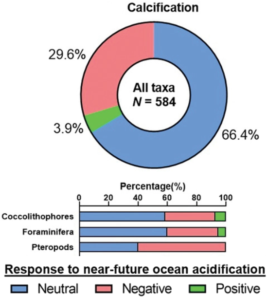
Fig. 7.33 The diverse response of CaCO₃ production rates of pelagic marine calcifiers to reductions in surface Ω. Figure from Leung et al. (2022).

Dissolution

The rate of dissolution of CaCO₃ in the surface ocean is a purely chemical process, and is a function of the saturation (Ω) of the waters. Dissolution rate is commonly formulated as:

\[\dv{\ce{CaCO_3}}{t} = [\ce{CaCO3}] k_{diss} \left( 1 - \Omega \right)^n\]

Where \(k_{diss}\) is a rate constant and \(n\) is an exponent that describes the reaction order of dissolution process. From this, we can calculate the fraction of CaCO₃ produced in the surface layer that has not dissolved at the base of the surface layer (\(f_{remaining}\)) as (Fig. 7.34):

\[f_{remaining} = e^{k_{diss} t (1 - \Omega)^n}\]

Where \(t\) is the amount of time for a sinking particle to reach the bottom of the surface layer. For this, we assume a particle sinking velocity of 10 m d^-1, and use the surface layer thickness of 100 m for the lolat box and 200m for the hilat box.

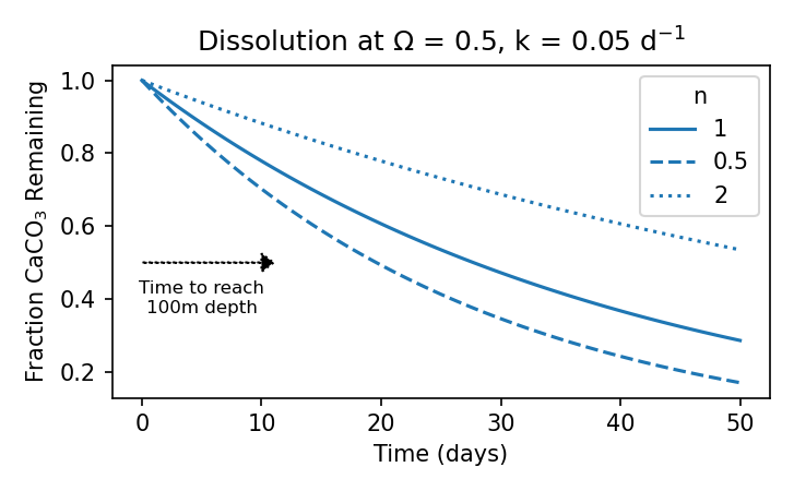
Fig. 7.34 The dissolution of CaCO₃ in under-saturated waters.

This equation would predict that there is no dissolution in supersaturated surface waters, which we know is not the case because of localised low-saturation regions that are generated by microbial activity in sinking particles. To account for this, we will assume that this local dissolution will effectively raise the ocean saturation state at which dissolution will begin, meaning that dissolution will begin when the surface water drops below a critical value of \(\Omega_{crit}\). Studies of the dissolution of CaCO₃ in the surface ocean have shown that the effective Ω values within these particles is around 2 units lower than in the surrounding seawater, so we will use an \(\Omega_{crit}\) of 3. Thus:

\[\begin{split}f_{remaining} = \begin{cases} e^{k_{diss} t (\Omega_{crit} - \Omega)^n} & \mathrm{for~\Omega < \Omega_{crit}} \\ 1 & \mathrm{for~\Omega > \Omega_{crit}} \\ \end{cases}\end{split}\]

Export

The final fraction of CaCO₃ exported from the surface to the deep ocean, \(f_{calc}\) is then:

\[\begin{split}f_{calc} &= f_{produced} ~ f_{remaining} \\ &= \begin{cases} 0.15 \Omega ~ e^{k_{diss} t (\Omega_{crit} - \Omega)^n} & \mathrm{for~\Omega < \Omega_{crit}} \\ 0.15 \Omega & \mathrm{for~\Omega > \Omega_{crit}} \\ \end{cases}\end{split}\]

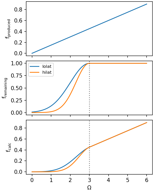
Fig. 7.35 The dependence of CaCO₃ production \((f_{produced})\), dissolution \((f_{remaining})\) and export \((f_{calc})\) on the saturation state of the surface ocean. Production increases linearly with saturation, while dissolution increases exponentially when Ω falls below a critical value of 3 (vertical dashed line).

Example Lab Report Scenario

Create a modified version of your model which includes the impact of ocean acidification on CaCO₃ export from the surface ocean (f_CaCO3). f_CaCO3 should be a function of the saturation state of aragonite in the surface ocean (Ω), which affects both the production of CaCO₃ in the surface ocean, and how much of the produced CaCO₃ is dissolved before it leaves the surface layer.

Model CaCO₃ production associated with biological productivity as a linear function of Ω:

\[ f_{production} = 0.15 \Omega_A \]

The fraction of this produced CaCO₃ that is exported from the surface ocean (f_remaining) should be calculated using an exponential decay function of the form:

\[\begin{split} f_{remaining} = \begin{cases} e^{k t (\Omega_{crit} - \Omega)^n} & when ~ \Omega_A < \Omega_{crit} \\ 1 & when ~ \Omega \geq \Omega_{crit} \end{cases} \end{split}\]

where \(k\) is the dissolution rate constant, \(n\) describes the reaction order of dissolution, \(t\) is the time a sinking particle remains in the surface ocean, and \(\Omega_{crit}\) is the saturation at which dissolution begins. Use values of \(k = 0.05\) g g^-1 d^-1, \(n = 2\) and \(\Omega_{crit} = 3\), which is greater than 1 to account for the impact of localised dissolution within sinking particles. To calculate the time it takes a sinking particle to reach the bottom of the surface layer, use a sinking velocity of 10 m d^-1.

Impact on Steady State Model

Example Lab Report: Part 1

Initialise your new model at the steady-state conditions of the unmodified model, and compare the evolution of the carbon system in the two models. Describe any significant differences and similarities.

If we have parameterised the impact of ocean acidification well, the steady-state of the modified model should be very similar to the unmodified model, because the unmodified model was already doing a good job of representing the system. We would expect any changes that are present to be limited to the carbon chemistry of the model, as f_CaCO3 only directly impacts TA and DIC in the model; it has no effect on temperature, salinity or nutrients.

In Fig. 7.36, we can see the differences between the carbon system in the original model and the new model including the sensitivity of f_CaCO3 to Ω. The steady state of the models is very similar. The largest difference is in the f_CaCO3 parameter itself, and consequently in the TA of the surface boxes. The value of f_CaCO3 in the lolat box is slightly higher than the original model (0.31 vs. 0.3), while the value in the hilat box is substantially lower (0.12 vs. 0.2). This causes TA in the lolat box to be slightly lower compared to the original model, while the TA in the hilat box is slightly higher. Deep TA is very slightly higher in the new model, which is caused by the larger size of the lolat box making it have a greater influence on the steady state value deep. The steady-state atmospheric pCO₂ is ~415 ppm in both models.

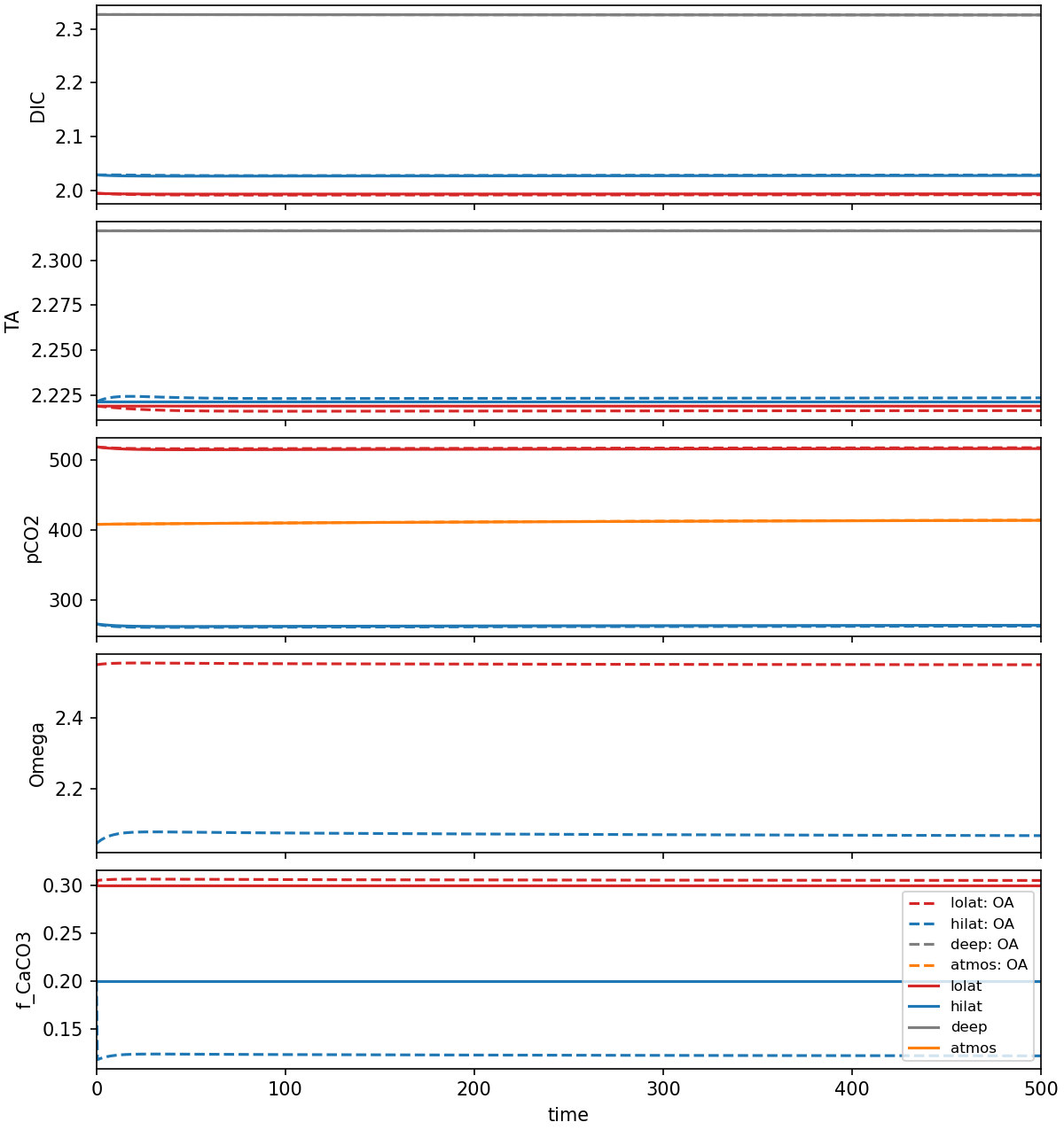
Fig. 7.36 The modified model compared to the unmodified model evolving to steady, initialised at the steady state conditions of the unmodified model. This shows that the steady state of the new model is very similar to the unmodified model, indicating that the parameterisation of f_CaCO3 is reasonable.

Overall, the similarity of the steady-state carbon system between the new model to the original model suggests that the addition of the ocean acidification feedback has only a small effect on the overall operation of the model under static conditions. This similarity suggests our parameterisation of ocean acidification is reasonable, and makes comparisons between the response of these models to perturbations straightforward - if the stead-states of the models were very different, it would be difficult to compare the response of the models to the same perturbation.

pCO₂ Release Experiment

Example Lab Report: Part 2

Conduct a CO₂ release experiment, where 8 PgC yr^-1 is released into the atmosphere for 200~years (model years 400-600). Run the model for a total of 3000 years, and examine the evolution of pCO₂, Ω, and CaCO₃ export over time compared to the unmodified model. Discuss the patterns you observe.

The influence of the new ocean acidification feedback becomes apparent when the model is perturbed by a large release of CO₂ into the atmosphere. In the scenario below (Fig. 7.37) we have released 8 PgC yr^-1 of CO₂ into the atmosphere for 200 years. There are two distinct phases in response of models to this perturbation:

1. During the CO₂ release (400-600 years) the surface ocean and atmosphere respond rapidly.

2. After year 600 the models gradually return to a new steady-state on a timescale consistent with ocean mixing processes.

The behaviour of the models diverges in both the rapid and long-term responses.

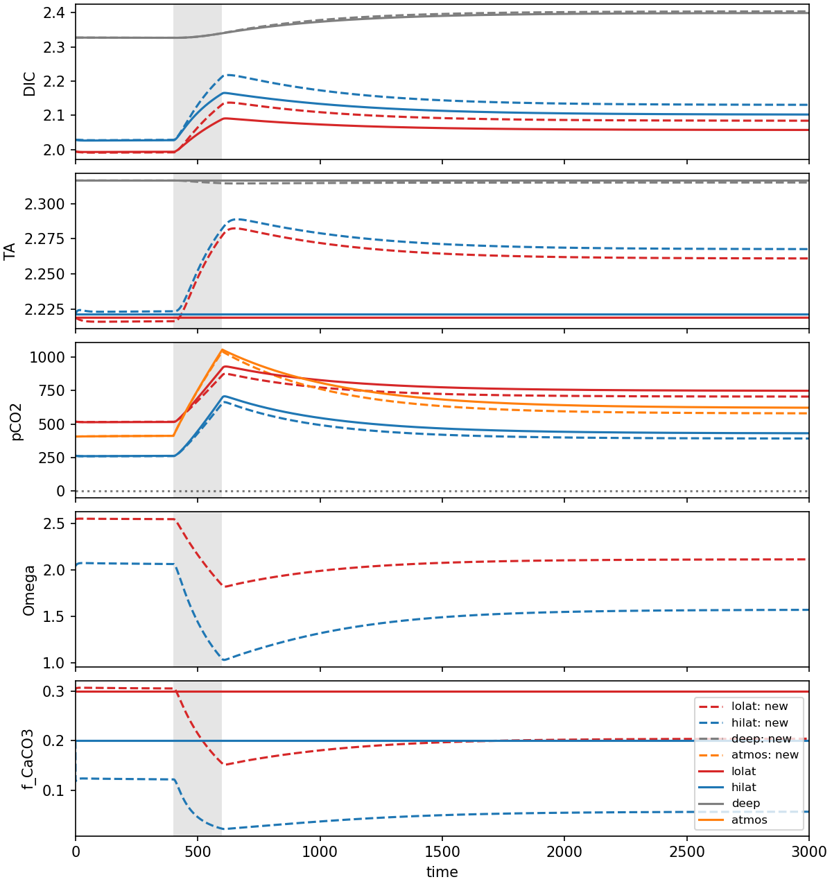
Fig. 7.37 The response of the modified and unmodified models to a CO₂ release experiment where 8 PgC yr^-1 are emitted during the grey shaded region. The horizontal dashed line in the Omega panel shows the value of Omega_crit where dissolution starts reducing the efficiency of CaCO₃ export from the surface ocean.

Rapid Response

During the CO₂ release, atmospheric pCO₂ increases approximately linearly, reaching a maximum of 1042 and 1057 ppm at the end of the emission period (year 600) in the new and original models, respectively. The peak pCO₂ is lower in the new model because of the large drop in f_CaCO3 in both surface boxes caused by the influx of CO₂ reducing \(\Omega\) in the surface ocean. The response of the hilat surface is particularly extreme, where CaCO₃ export almost stops completely (f_CaCO3 drops from 0.12 to 0.02) at the end of the perturbation. The reduced calcification in the surface ocean significantly elevates surface TA and, to a lesser extent, DIC, shifting the DIC equilibrium away from CO₂ and allowing the surface ocean to take up more of the CO₂, and thereby reducing the peak pCO₂ in the atmosphere. Before the perturbation TA was ~100 µmol kg^-1 higher in the deep than the surface boxes, which reduces to ~40 µmol kg^-1 immediately after the end of the perturbation, highlighting a significant redistribution of TA, and therefore DIC speciation, within the model.

At the end of the CO₂ release the majority of the disturbance is seen in the atmosphere and surface ocean. In the deep box, DIC is very slightly elevated, and TA is slightly reduced. This is because the deep box does not communicate directly with the atmosphere, and must rely on chemical, biological and mixing processes to transfer the effects of the perturbation in the atmosphere via the surface ocean. With this in mind, the difference in the response between the deep DIC and TA is interesting. The TA disturbance reaches a maximum in all boxes 20-30 years after the end of the CO₂ release experiment. This is because f_CaCO3 in the surface remains low for some time after the end of the perturbation, causing a prolonged period of reduced CaCO₃ export from the surface ocean. This prolonged reduction in export causes TA to continue to concentrate in the surface ocean until Ω begins to recover sufficiently to allow CaCO₃ export to resume.

Gradual Recovery

After the end of the perturbation, all the carbon system parameters gradually return to a new steady-state value which is somewhere between the starting value and the maximum disturbance reached at the end of the CO₂ release period. The notable exception to this trend is deep DIC, which stabilises to a new steady-state value that is substantially higher than the starting value. This indicates that a significant fraction of the emitted carbon is stored in the deep ocean in both models.

During this gradual recovery, f_CaCO3 and Ω recover to some degree in the surface boxes, but never reach pre-disturbance levels. This maintained lower calcification causes TA and DIC to remain elevated in the surface boxes in a 2:1 ratio, shifting surface DIC speciation away from CO₂, and causing more of the atmospheric CO₂ to be taken up by the surface ocean. As a result, the new model stores more of the emitted carbon in the ocean than the original - the deep ocean in the new model contains 74 PgC more than in the original model. This translates to 70% of the emitted carbon ends up in the deep ocean in the original model, and 74% in the new model.

The reduced CaCO₃ export in the new model provides a negative feedback on atmospheric pCO₂, which is not present in the original model. This has two main effects (Fig. 7.38):

1. The recovery to steady-state pCO₂ is faster in the new model than in the original model, with the maximum difference between the models ocurring at year ~1350, where pCO₂ in the new model is 50.4 ppm lower than in the original model.

2. The steady-state pCO₂ in the new model is 42 ppm lower than in the original model, because teh overall reduction in calcification in the new model allows more of the released CO₂ to be stored in the deep ocean.

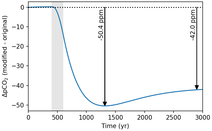
Fig. 7.38 The difference betweeen atmosphweric pCO₂ between the modified and original models after a CO₂ release experiment (8 PgC yr^-1 for 200 years in the grey bar).

Additional Factors

Example Lab Report: Part 3

What additional factors might influence how these patterns manifest in the real ocean? How might you test these additional factors in the model?

The implementation of the ocean acidification feedback used here assumes that marine calcifiers are uniformly influenced by decreased saturation. In reality, marine calcifiers exhibit a range of responses to ocean acidification, including suggestions that some increase calcification in response to elevated DIC (Fig. 7.33). The nature of the relationship used to link carbon chemistry and f_CaCO3 is therefore uncertain, and will cause the results of this model to vary. This could be evaluated by exploring a range of plausible relationships between model carbon chemistry and f_CaCO3. It is also unrealistic to model the impact of acidifcation purely as a function of aragonite saturation because numerous calcifiers make shells out of calcite, a more stable form of calcium carbonate. Switching to a calcite saturation state would reduce the magnitude of all of the impacts seen above.

A second important factor that might alter the patterns we see in the model is the interaction of calcification ‘ballasting’ the biological pump. Ballasting describes the increase in particle sinking speeds of marine particles which contain dense minerals, allowing them to sink faster and increasing the export of organic carbon from the surface ocean and the efficiency of the biological pump. If this were the case, the reduced biological pump efficiency associated with ocean acidification might drive an increase in atmospheric pCO₂ that could offset some or all of the reduction in pCO₂ associated with the calcification feedback. This could be tested by connecting the particle sinking velocity used above to f_CaCO3 in the model, and scaling \(\tau_P\) as a function of particle sinking speeds, as greater ballasting driven by f_CaCO3 would increase organic matter export rates and decrease the residence time of nutrients in the surface ocean.