7.2. The Solubility Pump

Key Points:

• The amount of CO₂ that dissolves in water strongly depends on the temperature of that water.

• Variations in CO₂ solubility and ocean circulation interact to drive the solubility pump.

• The solubility pump traps high-CO₂ water in the deep ocean.

• CO₂ reacts with water to create non-exchangeable Dissolved Inorganic Carbon (DIC) species.

• These reactions increase the amount of carbon that can dissolve into the water.

• The DIC species exist in an equilibrium with water pH, which is critical for understanding the ocean carbon budget.

The majority of carbon (~98%) in the ocean exists as Dissolved Inorganic Carbon (DIC). The DIC pool is the primary carbon reservoir in the ocean, and the chemical properties of DIC determine how much CO₂ the ocean can absorb. We’ll now look at how CO₂ and DIC are related.

CO₂ dissolves in water

We saw previously that CO_2(g) behaves like an ideal gas and dissolves from air into water until it reaches an equilibrium with CO_2(aq) described by Henry’s Law (7.1).

The solubility constant for CO₂, \(K_0\), depends strongly on temperature, and weakly on salinity (Fig. 7.7). This means that more gas will dissolve into colder, fresher water than warmer, saltier water.

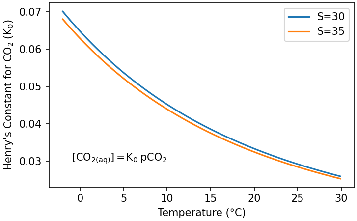
Fig. 7.7 Change in \(K_0\) with temperature and salinity.

As surface currents move from the equator towards the poles (e.g. along Western boundary currents like the Gulf Stream), the water loses heat to the atmosphere and cools down (Fig. 7.8).

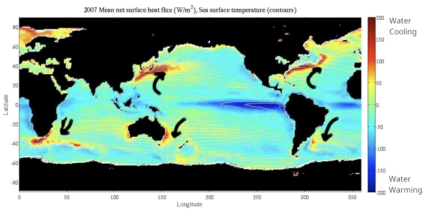
Fig. 7.8 Heat loss and absorption by the ocean. The ocean loses heat as warmer water moves to high latitudes, and gains heat as cool deep water rises to the surface in upwelling zones. Black arrows indicate major surface currents.

The drop in temperature causes \(K_0\) to increase (Fig. 7.7), allowing the water to take up more dissolved CO₂ at a given atmospheric pCO₂ (Fig. 7.9). The water reaches as a temperature minimum at its density maximum, just before it sinks to the deep ocean, which means that this sinking water has the highest [CO_2(aq)] of any surface water. The downwelling of cold, CO₂-rich water therefore removes carbon from the atmosphere.

Once in the deep ocean the water is isolated from the atmosphere until it upwells somewhere along the circulation path, 100s-1000s of years later. Consequently, upwelling zones bring CO₂-rich water to the surface, which is released to the atmosphere (Fig. 7.9) as the water warms and \(K_0\) decreases (Fig. 7.7).

This cycle, driven by the interaction of ocean circulation and changes in \(K_0\), is known as the solubility pump.

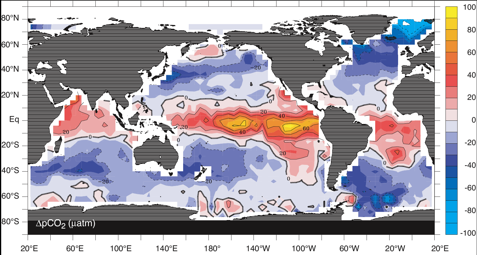
Fig. 7.9 The difference between surface ocean and atmospheric pCO₂. Notice that the ocean tends to take up CO₂ along the path or poleward surface currents (blue colours; e.g. North Atlantic), and release CO₂ in upwelling zones where carbon-rich water is brought to the surface and heated up (red colours; e.g. at the equator and in the North Pacific). The main patterns of uptake and release are similar to the patterns of water cooling and heating in Fig. 7.8. These patterns can be explained by the solubility pump, but the magnitude of the difference is much larger than predicted by Henry’s Law alone.

The solubulity pump explains first-order patterns of CO₂ uptake and release (Fig. 7.9), but is not enough to explain the high concentration of inorganic carbon in the ocean. If we take the entire range of \(K_0\) (0.02 to 0.07) at modern atmospheric pCO₂ (420 ppm), this only allows an equilibrium CO_2(aq) concentration of between 8.4-33.6 μmol kg^-1. Measurements of inorganic carbon in the ocean show that the actual concentration is on the order of 2000-2500 μmol kg^-1.

CO₂ reacts with water

There is more carbon in the ocean than we would expect based on gas solubility because CO_2(aq) reacts with water to form non-gaseous species that cannot exchange with the atmosphere. Once CO_2(g) is dissolved to CO_2(aq) it reacts with water to form a weak diprotic acid (an acid with two protons, H⁺) called carbonic acid. This acid dissociates to produce the Dissolved Inorganic Carbon (DIC) species:

(7.6)\[\mathrm{CO_{2(g)} \Leftrightarrow \underbrace{CO_{2(aq)}}_{dissolved~gas} + H_2O \Leftrightarrow \underbrace{H_2CO_3}_{carbonic~acid} \Leftrightarrow \underbrace{HCO_3^-}_{bicarbonate} + H^+ \Leftrightarrow \underbrace{CO_3^{2-}}_{carbonate} + 2H^+}\]

Where DIC is defined as the sum of these species in seawater:

Units!

Square brackets denote the concentration of a dissolved chemical species

(7.7)\[\begin{split}\mathrm{DIC} &= \mathrm{[CO_{2(aq)}] + [H_2CO_3] + [HCO_3^-] + [CO_3^{2-}]} \\ &= \mathrm{[CO_2^*] + [HCO_3^-] + [CO_3^{2-}]}\end{split}\]

where \(\mathrm{[CO_2^*] = [CO_{2(aq)}] + [H_2CO_3]}\) because carbonic acid is functionally absent in normal seawater - as soon as CO_2(aq) reacts with water the carbonic acid dissociates to form bicarbonate and a proton.

Note on CO₂*…

[CO₂^*] is a good approximation in most cases, but be aware that the reaction of CO_2(aq) with water is much slower than the subsequent dissociation reactions because it requires breaking strong C-O bonds, whereas the dissociation involves adding/removing weakly-bound protons (H⁺). This means that the CO₂ approximation may start to break down in dynamic systems where DIC speciation is far from equilibrium with CO_2(aq). This can become important when considering rapid ocean-atmosphere interactions, because CO_2(aq), rather than than H₂CO₃, is the species that exchanges with CO_2(g) in the atmosphere. However, for our purposes, the CO₂ approximation is a good one.

Because CO_2(aq) is the only species that exchanges with CO_2(g) in the atmosphere, the speciation of DIC is critical in determining how much DIC the ocean will contain at a given atmospheric pCO₂. From Eq (7.6) we see that DIC speciation will depend on the concentration of each of the DIC species and H⁺ in the water. The concentration of H⁺ is described by the pH of the water (pH = -log₁₀[H⁺]), which tells us that the concentration of the DIC species in seawater is a function of pH (Fig. 7.10).

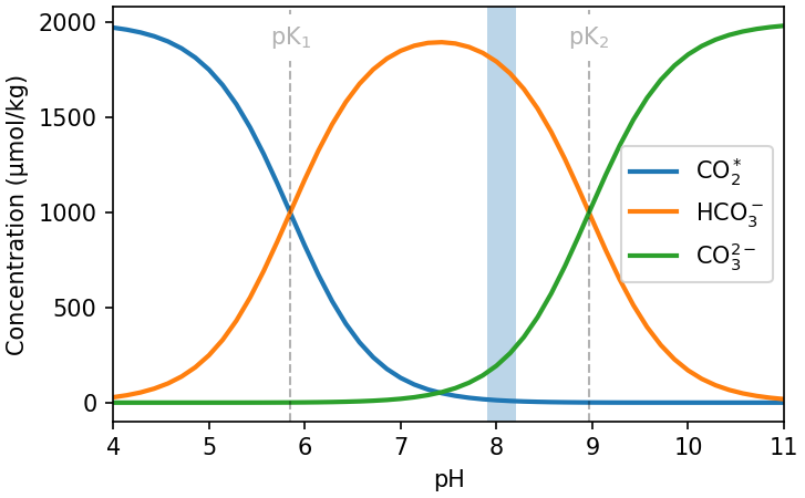
Fig. 7.10 The concentration of DIC species in seawater as a function of pH. The vertical blue bar shows the typical pH range in surface ocean water, and vertical dashed lines show the locations of the equilibrium constants that define the dissociation of DIC in seawater.

At a typical surface seawater pH of ~8.1 only ~0.5% of the DIC is in the form of CO_2(aq) (Fig. 7.10). Most DIC exists as the non-exchangeable species bicarbonate and carbonate. For a typical surface ocean DIC of ~2000 μmol kg^-1, this corresponds to a CO₂ concentration of ~10 μmol kg^-1, which is within range of the [CO_2(aq)] concentration predicted by Henry’s Law for 420 ppm (8-34 μmol kg^-1 between 0-30 °C)!

The reaction of CO_2(aq) with water explains why the concentration of DIC in seawater is so much higher than predicted by gas solubility.

DIC Speciation

The speciation of DIC shown in Fig. 7.10 is described by acid-base equilibria defined by the equilibrium constants \(K_1\) and \(K_2\):

(7.8)\[\begin{split}\mathrm{CO_{2}^*} &\overset{K_1}{\Leftrightarrow} \mathrm{HCO_3^- + H^+} \\ \mathrm{HCO_3^-} &\overset{K_2}{\Leftrightarrow} \mathrm{CO_3^{2-} + H^+}\end{split}\]

Where \(K_1\) and \(K_2\) are defined as:

(7.9)\[\begin{split}K_1 &= \mathrm{\frac{[H^+][HCO_3^-]}{[CO_2^*]}} \\ K_2 &= \mathrm{\frac{[H^+][CO_3^{2-}]}{[HCO_3^-]}}\end{split}\]

These \(K\) values are sensitive to temperature, salinity and pressure. The speciation of DIC and pH will therefore shift as the physical properties of the water change.

Temperature, salinity and pressure…

The temperature and pressure dependence of \(K_1\) and \(K_2\) are related to the thermodynamics of the dissociation reactions. Varying the temperature and pressure of the environment alters the standard free energy of these reactions, which in turn alters the equilibrium constants. The effect of salinity is more complex, and comes about because seawater is not an ideal solution, so ion concentration deviates significantly from ion activity. The activity of ions in seawater is reduced by ion-ion interactions, which varies with the concentration of individual ions, the overall ionic strength, and the temperature of the solution. Many attempts have been made to calcualte the impacts of salinity and ion-ion interactions on equilibrium constants in seawater (for example the Pitzer equations, Debye-Hückel theory and the Davies equation), but none of these attempts do a perfect job. In practice, we calculate \(K_1\) and \(K_2\) using empirical functions that have been fitted to careful measurements of DIC speciation in seawtaters over a range of temperature, salinity and pressure.

The influence of temperature and pressure is thermodynamic, because these both alter the free energy of the reaction. The influence of salinity is more complex, and comes from ion-ion interactions in seawater altering the activity of ions in solution. The details of these sensitivities are beyond the scope of this course, but be aware that temperature tends to have a larger influence on \(K\) values than salinity across the range of these values found in the oceans.

The definitions of \(K_1\) and \(K_2\) can be combined with the expression for DIC (7.7) to calculate the concentration of each dissolved DIC species as a function of [DIC], pH and the equilibrium constants:

[CO₂*] derivation…

\[\begin{split} \begin{align} DIC &= [CO_2^*] + [HCO_3^-] + [CO_3^{2-}] \\ &= [CO_2^*] + [HCO_3^-] + \frac{K_2 [HCO_3^-]}{[H^+]} & \mathrm{substitute ~ [CO_3^{2-}] ~ using ~ K_2} \\ &= [CO_2^*] + \frac{K_1[CO_2^*]}{[H^+]} + \frac{K_2 K_1 [CO_2^*]}{[H^+]^2} & \mathrm{substitute ~ [HCO_3^{-}] ~ using ~ K_1} \\ &= [CO_2^*] \left( 1 + \frac{K_1}{[H^+]} + \frac{K_2 K_1}{[H^+]^2} \right) & \mathrm{separate ~ [CO_2^*]} \\ [CO_2^*] &= \frac{DIC}{1 + \frac{K_1}{[H^+]} + \frac{K_1K_2}{[H^+]^2}} & \mathrm{solve ~ for ~ [CO_2^*]} \end{align} \end{split}\]

(7.10)\[\begin{split}\mathrm{[CO_2^*]} &= \frac{\mathrm{[DIC]}}{1 + \frac{K_1}{\mathrm{[H^+]}} + \frac{K_1K_2}{\mathrm{[H^+]}^2}} \\ \mathrm{[HCO_3^-]} &= \frac{\mathrm{[DIC]}}{1 + \frac{\mathrm{[H^+]}}{K_1} + \frac{K_2}{\mathrm{[H^+]}^2}} \\ \mathrm{[CO_3^{2-}]} &= \frac{\mathrm{[DIC]}}{1 + \frac{\mathrm{[H^+]}}{K_2} + \frac{\mathrm{[H^+]}^2}{K_1K_2}} \\\end{split}\]

The values of the equilibrium constants \(K_0\), \(K_1\) and \(K_2\) have been carefully determined for seawater, and can be calculated as a function of temperature, salinity and pressure. At standard salinity and temperature (35, 25 °C) and 1 atmosphere pressure (surface seawater), these K and pK (-log₁₀K) are:

	\(K\)	\(pK\)
\(K_0\)	\(2.839 \times 10^{-2}\)	1.547
\(K_1\)	\(1.422 \times 10^{-6}\)	5.847
\(K_2\)	\(1.082 \times 10^{-9}\)	8.966

Where the pK values denote the pH at which the species are present in equal concentrations (Fig. 7.10).

Solving the DIC system…

We’ve now seen that knowing the concentration of DIC in seawater alone is not enough to understand ocean carbon - we also need to know the state of DIC speciation. How do we determine this?

The equilibrium equations in (7.9) define a system of two equations with four unknowns (\([CO_2^*], [HCO_3^-], [CO_3^{2-}] and [H^+]\)). To determine the concentration of an individual DIC species we therefore need to know two of these variables.

In reality only one of these variables, pH, can be practically measured in seawater, which presents a problem. There are, however, two other properties that can be readily measured related to ocean carbon: DIC contencentration, and Total Alkalinity \((TA = 2 [CO_3^{2-}] + [HCO_3^-] + [minor~bases] + [OH^-] - [H^+])\), which is the sum of the charge of weak bases in seawater (don’t worry about this - it’s far beyond the scope of this course!). We now have four equations and six unknowns, but three of those unknowns are relatively easy to measure in seawater.

DIC, pCO₂ and pH

In Fig. 7.10 we show the concentration of the DIC species changing as a function of water pH, but this is only true for a fixed DIC concentration at constant temperature, salinity and pressure. You can see from (7.8)-(7.10) that the concentration of each DIC species and [H⁺] (and therefore pH) exist in an equilibrium, with the state of that equilibrium is defined by the \(K\) values. This means that if any component of the system is changed, all parts of the system will adjust to reach a new equilibrium state.

This has two important consequences that are relevant to our understanding of ocean carbon:

1. pCO₂ and DIC are not linearly related

Increasing pCO₂ raises the concentration of [CO₂*], as defined by Henry’s Law. The majority of this CO₂* then reacts with water to form non-exchangeable DIC species, allowing the ocean to absorb additional CO_2(g) from the atmosphere. This causes the total increase in DIC per unit pCO₂ to be much greater than the increase in [CO₂*] alone, ‘amplifying’ the effect of solubility pump.

The amplifying effect of DIC speciation is not uniform - it depends on the starting state of the DIC equilibrium, and temperature and salinity which set the \(K\) values (note we can ignore pressure here, because atmospheric exchange only happens at the surface). The new equilibrium state at higher pCO₂ has a reduced pH, which alters the balance of DIC species to favour [CO₂*]. Because more of the DIC pool exists as CO₂*, the capacity for DIC to store additional carbon over the prediction of Henry’s Law is reduced at higher pCO₂.

These mechanisms combine to drive a non-linear relationship between pCO₂ and DIC, as we can see in Fig. 7.11.

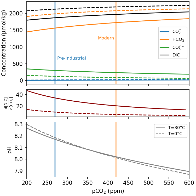
Fig. 7.11 The change in DIC concentration and speciation (top), pH (bottom) and the relative change in DIC compared to [CO₂] (middle) in warm and cold water as pCO₂ increases. Because CO₂ reacts with water, much more DIC is stored in seawater than we would expect based on Henry’s Law, driving a much greater increase in dissolved carbon as pCO₂ increases. However, because the equilibrium state of the DIC system changes as pCO₂ increases, the size of this amplifying effect decreases at high pCO₂. This leads to the non-linear relationship between pCO₂ and DIC observed here. The difference between high and low temperature water is driven by differences in the underlying speciation constants. Vertical lines show representative pre-industrial and modern pCO₂ values, highlighting the drop in surface ocean pH that has already occurred in the last ~200 years.

2. pCO₂ is negatively correlated with pH

Increasing pCO₂ decreases ocean pH in a process known as Ocean Acidification (Fig. 7.11). This follows directly from (7.7), where we see that the immediate dissociation of carbonic acid releases a proton into the ocean. The majority of these protons will react with CO₃^2- to form HCO₃^-, but the new equilibrium reached will be at a lower overall pH, with consequently different DIC speciation (towards the left in Fig. 7.10). This reduction CO₃^2- will become particularly important when considering The Carbonate Pump.

Conversely, any process that independently alters the pH of the ocean will change the speciation of DIC, allowing the surface ocean to take up or release CO₂. This becomes particularly important when considering the impact of biological processes, and The Carbonate Pump.

Modelling the Solubility Pump

To include the solubility pump in our model, we must:

1. Add a box to represent the atmosphere.

2. Parameterise the exchange of CO₂ between the atmosphere and the surface ocean.

3. Track the speciation of DIC in the surface ocean.

4. Track the concentration of DIC.

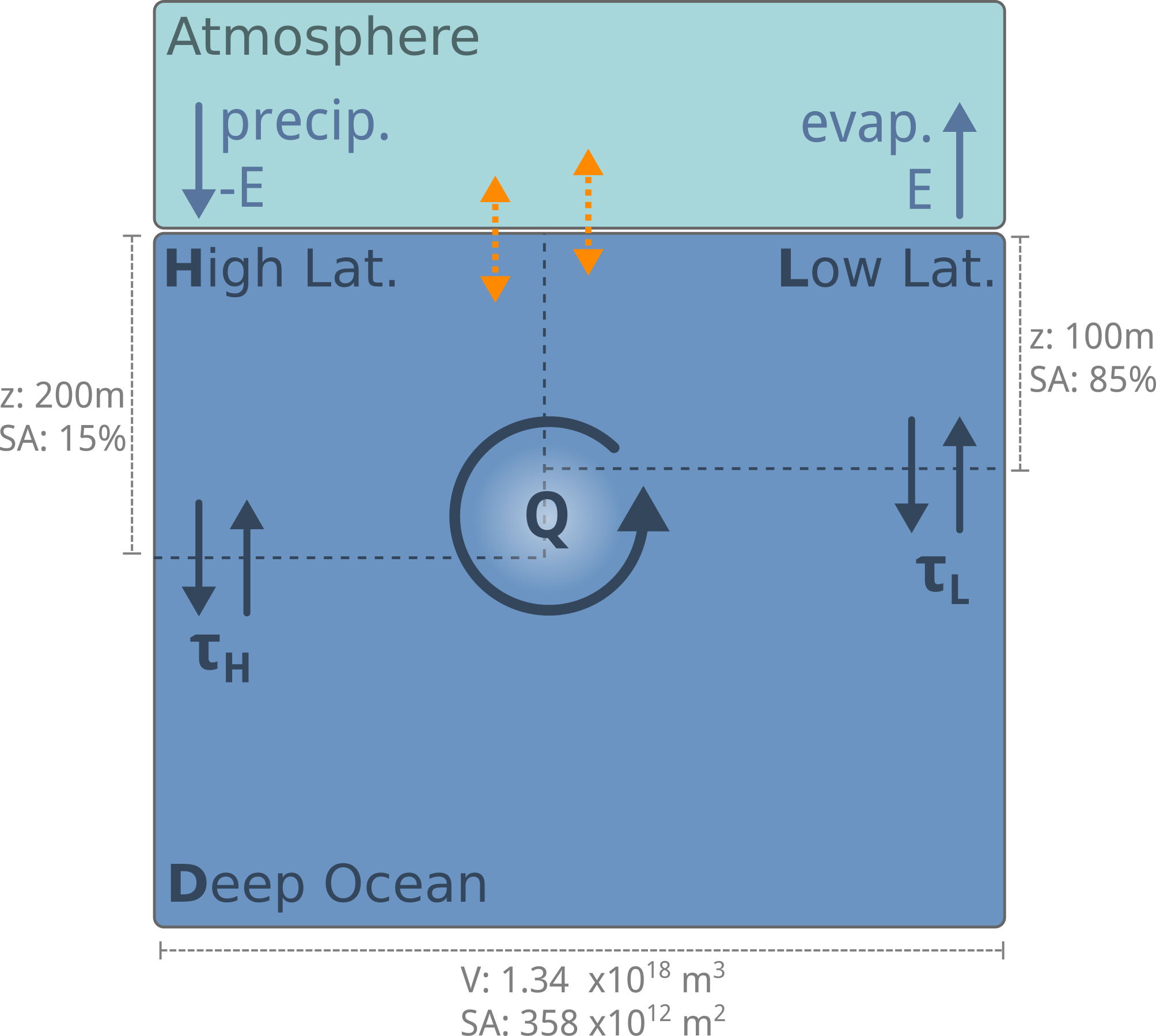
Fig. 7.12 To model the solubility pump, we need to include the exchange of CO₂ between the ocean and atmosphere, the conservative transport of DIC through the ocean interior, and the speciation of DIC in the surface ocean.

1. The Atmosphere

We will model the atmosphere as a single, well-mixed box that overlies both surface ocean boxes. This is an OK approximation because the processes of atmospheric mixing are much faster than the processes of ocean mixing. Our atmosphere will have a pCO₂, which is related to the number of moles of CO₂ in the atmosphere by:

(7.11)\[n_{CO2} = pCO_2~n_{air}\times 10^{-6}\]

where \(n_{air}\) is the number of moles of air in the atmosphere and \(pCO_2\) is in ppm. We can also calculate the mass of carbon in the atmosphere:

(7.12)\[m_{CO2} = n_{CO2} 12\]

where 12 is the atomic mass of carbon. For a pCO₂ of 400 ppm with \(n_{air}\) of 1.736x10²⁰, this yields a total mass of ~830 GtC in out model atmosphere.

2. Ocean-Atmosphere Exchange

We will model exchange in the atmosphere by allowing CO₂ in each surface box to equilibrate with the overlying atmosphere with a characteristic timescale, \(\tau^{CO2}\), which defines how quickly CO₂ in a surface box will equilibrate with pCO₂ in the overlying atmosphere (Fig. 7.6). This allows us to calculate the number of moles of C moving from the atmosphere into one of the surface boxes as:

Units!

\(K_0 pCO_2\) is in units of \(\mu mol~kg^{-1}\) if \(pCO_2\) is given in ppm. This therefore has to be multiplied by water density (~1025 kg m^-3) to convert to a volume concentration (\(\mu mol~m^{-3}\)), and a factor of \(10^-6\) to convert to \(\mathrm{mol~m^{-3}}\) to match \([CO_2]_i\).

(7.13)\[\dv{DIC_{CO2,i}}{t} = - \left. \underbrace{\frac{V_i}{\tau^{CO2}_i}}_{\mathrm{m^3~yr^{-1}}} \left( \underbrace{[CO_2]_i - K_{0,i} ~ pCO_2 ~ \rho_i ~ 10^{-6}}_{\mathrm{mol~m^{-3}}} \right) \middle/ V_i \right.\]

Where \(i\) is either of the surface boxes (\(L, H\)).

Conversely, the change in \(pCO_2\) of the atmosphere can be calculated as:

(7.14)\[\dv{pCO_2}{t} = \sum_{i=L,H} \left(\frac{V_i}{\tau^{CO2}_i} \left([CO_2]_i - K_{0,i} ~ pCO_2 ~ \rho_i ~ 10^{-6} \right) \right) \times 10^{6} / n_{air}\]

Where \(n_{air}\) is the number of moles of air in the atmosphere, and \(10^6\) converts to ppm.

To calculate the ocean-atmosphere flux, we need to know both the concentration of DIC and the state of DIC speciation to determine \([CO_2]_i\). We can track the transport of DIC just like any other conservative tracer (7.2), but keeping track of DIC speciation is a bit more complicated…

3. DIC Speciation

Above we calculated DIC speciation as a function of pH and the speciation constants \(K_1\) and \(K_2\), so can we use pH to model DIC speciation? Unfortunately, pH is not a conservative quantity. The \(K\) values for DIC speciation are sensitive to temperature, salinity and pressure, which also make pH sensitive to these parameters. This allows pH to change based on the physical properties of the box, so the total amount of \(H^+\) in the entire model is not constant - pH is not conservative. To track DIC speciation, we need a conservative quantity that, along with DIC, can be used to calculate the concentration of CO₂ in each surface box.

This conservative quantity is Total Alkalinity (TA), which is tricky concept that is beyond the scope of this course. For our purposes, it is sufficient to know that TA is approximately defined as:

(7.15)\[\mathrm{TA \approx 2[CO_3^{2-}] + HCO_3^- + [...] - [H^+]}\]

And be aware that:

• TA is conservative

• TA and DIC together can be used to calculate aqueous carbon speciation (Fig. 7.13).

• From (7.15), we can see that adding/removing CO₂ does not change TA because \(\mathrm{CO_2 + H_2O \rightarrow HCO_3^- + H^+}\), which cancel out in the definition of TA.

In practicals, you will use a python package to calculate DIC speciation.

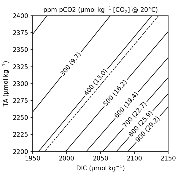
Fig. 7.13 DIC and TA can be combined to calculated pCO₂ and [CO₂] at a given temperature, salinity and pressure.

No but what actually is TA?!

TA has multiple definitions from different fields. TA is not the opposite of acidity, although increasing TA will also increase pH. For a chemist, TA is “a measure of the excess bases (proton acceptors) over acids (proton donors), and is operationally defined by the titration with H⁺ of all weak bases present in the solution” (Sarmiento & Gruber, 2006). In practical terms, it is the moles of H⁺ you must add to a kg of seawater to reach the equivalence point where [H⁺] = [HCO₃^-]. For an oceanographer, “TA is equal to the charge difference between conservative cations and anions”, so is a measure of the charge imbalance of seawater. It can also be thought of as the ‘buffering capacity’ of water, as higher alkalinity water has more proton acceptors so can better resist changes in pH.

If you really want to know the details, section 1.2 of Zeebe & Wolf-Gladrow (2001) provides a comprehensive overview… but you really do not need to know this for QES!

As no processes in our model currently modify TA (but they will soon), we can model TA using only the equations for conservative tracer transport in (7.2).

4. DIC Concentration

Now we have a way to keep track of DIC speciation, we can calculate the concentration of CO₂ in each surface box as:

\[[CO_2]_i = f(DIC_i, TA_i, T_i, S_i)\]

This allows us to model DIC as a conservative tracer (7.2), with additional terms for the exchange of CO₂ with the atmosphere in the surface boxes:

(7.16)\[\begin{split}\dv{DIC_L}{t} &= [\mathrm{transport}] - \frac{1}{\tau^{CO2}_L} ([CO_2]_L - K_{0,L} ~ pCO_2 ~ \rho_L ~ 10^{-6} ) \\ \dv{DIC_H}{t} &= [\mathrm{transport}] - \frac{1}{\tau^{CO2}_H} ([CO_2]_H - K_{0,H} ~ pCO_2 ~ \rho_H ~ 10^{-6}) \\ \dv{DIC_D}{t} &= [\mathrm{transport}]\end{split}\]

where \([\mathrm{transport}]\) represents the conservative transport terms from (7.2). Note that the deep box is only affected by transport terms because it does not exchange CO₂ with the atmosphere.