6.9. Thermohaline Circulation

In the previous section, we examined the shallow circulation that develops in the upper \(\sim 100\)m of ocean in response to wind forcing. In this section, we will examine the deep Thermohaline Circulation that develops in response to wind forcing and surface heating/cooling and evaporation/precipitation.

In earlier lectures, we noted that strong poleward-flowing currents (including the Gulf Stream) develop on the western sides of the ocean basins and that these transport significant amounts of heat from low to high latitudes. Also recall from Fig. 6.13 the curious observation that the mean sea level is higher on the western sides of ocean basins. We will start by quantitatively explaining both of these features of the large-scale ocean circulation. A key insight that underlies the theory that we will discuss is that the Coriolis parameter, \(f\) varies with latitude (recall that \(f=2\Omega \sin \theta\) where \(\theta\) is the latitude.

We start by integrating Eq. (6.35) over the full ocean depth where \(z=-H\) represents the seafloor and \(z=0\) is the ocean surface:

(6.42)\[\frac{\partial \overline{\mathbf{u}}}{\partial t} + f\hat{\mathbf{z}}\times \mathbf{u} = -\frac{1}{\rho}\nabla \overline{p} - \overline{g}\hat{\mathbf{z}} + \nu \left.\frac{\partial \mathbf{u}}{\partial z}\right|_{-H}^0,\]

where an overbar denotes a vertical derivative from \(z=-H\) to \(z=0\). As before, we will look for steady solutions. For simplicity, let’s assume as we did before that the wind stress is aligned with the \(x\)-direction, \(\mathbf{\tau}^w=\tau^w \hat{\mathbf{x}}\). For now, we will also neglect the viscous stress at the bottom of the ocean (\(z=-H\)). We will revisit this later. The horizontal components of Eq. (6.42) are

(6.43)\[-f\overline{v} = -\frac{1}{\rho} \frac{\partial \overline{p}}{\partial x} + \frac{\tau^w}{\rho},\]

(6.44)\[f\overline{u} = -\frac{1}{\rho} \frac{\partial \overline{p}}{\partial y}\]

We can eliminate the pressure by cross-differentiating Eqns. (6.43) and (6.44). When we do this, it is important to remember that \(f\) is a function of \(y\) since it varies in the north/south direction. The result is

(6.45)\[f\left(\frac{\partial \overline{u}}{\partial x}+ \frac{\partial \overline{v}}{\partial y}\right) + \overline{v}\frac{df}{dy} = -\frac{\partial}{\partial y}\left(\frac{\tau^w}{\rho}\right).\]

From the integral of the mass conservation (continuity) equation (Eq. (6.40)), we see that the first term in parentheses is equal to the difference between the vertical velocity at the bottom and top of the ocean. We can safely assume that both of these are zero and hence the first term in Eq. (6.45) vanishes and we are left with

(6.46)\[\overline{v} \frac{df}{dy} = -\frac{\partial}{\partial y}\left(\frac{\tau^w}{\rho}\right).\]

This equation is often referred to as Sverdrup balance after Harold Sverdrup who first derived it.

Eq. (6.46) is remarkable. Counter-intuitively, it tells us that the north/south component of the depth-integrated velocity, \(\overline{v}\) is related to the north/south derivative of the \(x\)-component of the wind stress. In the Northern Hemisphere subtropics, \(\partial \tau^w/\partial y>0\), and hence Eq. (6.46) predicts southward depth-integrated flow (\(\overline{v}\)) in this region. Note that this is somewhat different from the flow that we got in the previous section, but there we were only considering the flow in the upper ocean, whereas Eq. (6.46) applies to the depth-integrated velocity.

We can use Eq. (6.46) to see why the sea surface is higher on the western sides of ocean basins at mid-latitudes. Recall from our earlier lectures that the Rossby number associated with global-scale ocean circulation is very small, and hence we expect ocean currents on this scale to be in geostrophic balance. In the ocean, we related the currents to gradients in the sea surface height. If we integrate the geostrophic balance relation from \(z=-H\) to \(z=0\), we get

(6.47)\[f\overline{v} = gH\frac{\partial \eta}{\partial x}.\]

Using Eq. (6.47) in Eq. (6.46) gives

\[\frac{gH}{f}\frac{\partial \eta}{\partial x} \frac{d f}{d y} = -\frac{\partial}{\partial y}\left(\frac{\tau^w}{\rho}\right).\]

Since \(df/dy>0\), regions where \(\tau^w\) increases with latitude will have \(\partial \eta/\partial x<0\). In other words, the sea surface height decreases in the eastwards direction and hence the sea surface height is higher on the western sides of the ocean basins at mid-latitudes.

At this point we encounter a paradox: Eq. (6.46) tells us that the depth-integrated ocean currents are to the south in the Northern Hemisphere in the subtropics. However, the water cannot simply build up near the equator - somehow it must return to the north. We anticipate that the water will return to the north near the coastline where the current will experience extra drag. Specifically, we will add an additional term to Eq. (6.43) and Eq. (6.44) to represent drag on the boundary currents. Following early work by Stommel, we will assume that the drag force is a linear function of the depth-integrated velocity so that Eqns. (6.43) and (6.44) can be written

(6.48)\[-f\overline{v} = -\frac{1}{\rho} \frac{\partial \overline{p}}{\partial x} + \frac{\tau^w}{\rho} - r \overline{u},\]

(6.49)\[f\overline{u} = -\frac{1}{\rho} \frac{\partial \overline{p}}{\partial y} -r \overline{v}\]

where \(r\) is a constant drag coefficient. If we follow the same steps as above, we arrive at a new version of Eq. (6.46):

(6.50)\[\overline{v}\frac{df}{dy} = -\frac{\partial}{\partial y}\left(\frac{\tau^w}{\rho}\right) - r \left(\frac{\partial \overline{v}}{\partial x} - \frac{\partial \overline{u}}{\partial y}\right).\]

In the boundary current regions, we expect the current to be predominately north/south and for derivatives in \(x\) to be larger than derivatives in \(y\). Hence, we expect that \(|\partial \overline{v}/\partial x| \gg |\partial \overline{u}/\partial y|\). If the boundary current occupies a relatively narrow region near the coast (compared to the width of the ocean basin), then the term involving the wind stress in Eq. (6.50) must be small compared to the left hand side. Hence, we have approximately

(6.51)\[\overline{v}\frac{df}{dy} = -r \frac{\partial \overline{v}}{\partial x}.\]

Since \(df/dy>0\), Eq. (6.51) implies that a northward velocity (\(v>0\)) must be accompanied by \(\partial v/\partial x < 0\). This scenario can only work on the western side of the ocean basins.

To obtain a more intuitive physical explanation for the formation of western boundary currents, we can invoke conservation of angular momentum. On a rotating planet, conservation of angular momentum tells us that the sum of the angular momentum associated with spinning currents and the planet’s rotation must be conserved in the absence of external forces. If we imagine looking down at the Earth from above the north pole, the Earth will appear to rotate counter-clockwise. The vertical component of this rotation decreases with latitude. When wind acts to add clockwise spin to the water - as is the case in the Northern Hemisphere subtropics - the water must move towards the equator to conserve its angular momentum. This is an explanation for Sverdrup balance. The problem is that the Earth’s angular momentum will be re-gained when the water returns to the north. In order to maintain a steady circulation, the drag within the boundary current must decrease the clockwise spin in order to counter-balance the spin added by the wind.

We can make this argument more quantitative by introducing the concept of vorticity. The vorticity can be defined as

\[\omega = \frac{\partial v}{\partial x} - \frac{\partial u}{\partial y},\]

and this is a measure of the spin of a parcel of water. When \(\omega>0\) the water is spinning counter-clockwise. Notice that the vorticity appears on the right hand side of Eq. (6.50). In fact, if we had kept the time-derivative terms, then Eq. (6.50) would be

(6.52)\[\frac{\partial \overline{\omega}}{\partial t} + \overline{v}\frac{df}{dy} = -\frac{\partial}{\partial y}\left(\frac{\tau^2}{\rho}\right) - r \overline{\omega}.\]

Hence, Eq. (6.52) is an evolution equation for the vorticity. In the absence of external forcing (if the RHS of Eq. (6.52) is zero) then if the fluid moves to the south \(\overline{v}<0\), then the vorticity must increase. This is a mathematical statement of conservation of angular momentum. In order to compensate for negative vorticity input by the wind in the Northern Hemisphere subtropics, the bottom drag must act to add positive vorticity in the boundary current. A boundary current on the eastern side of the basin would have positive vorticity, and hence the bottom drag term \(-r \omega < 0\), which is in the wrong sense. However, a boundary current on the western side of the basin would have negative vorticity, and the bottom drag would impart positive vorticity as needed to balance the negative vorticity input by the wind.

Unlike the shallow wind-driven ocean circulation that we discussed in the previous lecture, the western boundary currents tend to be quite deep. For example, the Gulf Stream extends to depths below 1000m. However since the upper ocean is much warmer than the deep ocean (see Fig. 6.4, most of the poleward heat flux occurs near the surface. To a large extent, the western boundary currents are responsible for the poleward near-surface heat flux (the upper advective flux in the Stommel model). This represents one component of the Thermohaline Circulation.

As the western bondary currents flow polewards, they lose heat (see Fig. 6.22) and the density of the water increases. The water eventually becomes dense enough to sink to the deep ocean. This sinking occurs in relatively small areas through a process called deep convection. The water then spreads throughout the ocean interior and very slowly returns up to the surface. The water involved in a closed loop of the Thermohaline Circulation could travel extremely long distances, as sketched in Fig. 6.23 and Fig. 6.4. It can take more than 1000 years for a parcel of water to complete this circuit. This long timescale is very important for the climate system. Since the ocean is a major reservoir of heat and carbon, the climate system has a very long `memory’. By burning fossil fuels, we are adding antropogenic carbon to the ocean. Some of this carbon will remain in the ocean for more then 1000 years!

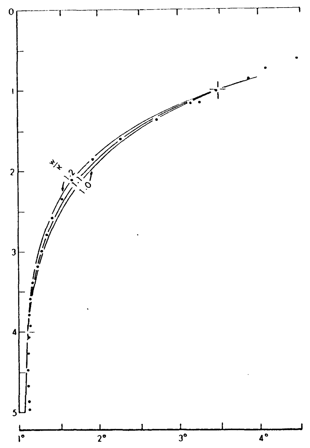
Fig. 6.33 Temperature measurements from the eastern Pacific ocean. The vertical axis indicates depth in km. From Munk, 1966.

Based on this description, we might expect the deep ocean to fill up with the very cold water that sinks at high latitudes. To some extent this is true, but the as shown in Fig. 6.33, the temperature in the ocean interior is non-uniform and decreases gradually with depth. A remaining question is: if the cold water at the bottom of the ocean is gradually moving up, what is the source of heat that prevents the deep ocean from filling with the coldest water. Sunlight only penetrates the upper 10’s of meters, so solar heating cannot explain the observed temperature profile.

A solution to this problem was proposed by Munk, 1966. Munk proposed that downward mixing of heat by small-scale turbulence balances the upward advection of cold water. To model this, he used an advection/diffusion equation for a vertical profile of temperature, \(T(z,t)\) of the form

\[\frac{\partial T}{\partial t} + w\frac{\partial T}{\partial z} = \kappa \frac{\partial^2 T}{\partial z^2}.\]

At steady state, \(\partial T/\partial t=0\) and advection should balnce diffusion:

\[w\frac{\partial T}{\partial z} = \kappa \frac{\partial^2 T}{\partial z^2}.\]

If \(\kappa\) and \(w\) are constant, then this leads to solutions where the density is an exponential function of depth. Fig. 6.33 shows several exponential curves with different values of \(w/\kappa\) (labelled in units of km\(^{-1}\)).

Using radiocarbon data and estimates of sinking rates at high latitudes, Munk estimated that about \(Q\simeq 25 \times 10^{6} \mbox{m}^3/\mbox{s}\) upwell through a fixed depth globally. If we assume that this water upwells uniformly across the ocean area which is about \(A\simeq 4 \times 10^{14} \mbox{m}^2\), we get \(w=Q/A \simeq 6 \times 10^{-8} \mbox{m}/\mbox{s}\). Note that this is velocity is far too slow to measure directly.

Based on these estimates for the upwelling velocity and emprical fits to the temperature profiles in Fig. 6.33, Munk estimated that \(\kappa\simeq 10^{-4}\mbox{m}^2/\mbox{s}\). This is about 1000 times larger than the molecular diffusivity of heat in water, so eddying fluid motion is needed to accomplish this heat flux. In recent years, oceanographers have attempted to measure \(\kappa\) using tracers or by directly measuring turbulent motion. This work has converged on estimates near \(\kappa \simeq 10^{-5} \mbox{m}^2/\mbox{s}\), which is an order of magnitude smaller than Munk’s estimates. The reasons for this discrepancy still remain uncertain. One possbility which has recieved a lot of attention is that the upwelling does not occur uniformly throughout the ocean. Reserach into this question is still ongoing.

In the next section we will describe a box model that more explicitly represents the Thermohaline Circulation by adding a deep box to the Stommel model. This will also be the focus of the computing practical work. We will then use this model to study the ocean’s carbon system.