2.4. Groundwater challenges and sustainable groundwater#
We have discussed the importance of groundwater systems, how groundwater moves (and why it can move uphill), and how we can test for and figure out the key aspects that influence groundwater flow, which includes pumping tests. Together these give us a good sense of how to calculate groundwater velocity and the energy required to move groundwater. There are several environmental challenges that face Earth’s groundwater systems, not least of which is the fact that we are removing groundwater faster than it can recharge. We can see this in global maps of groundwater depletion (Fig. 2.23). Groundwater depletion refers to the permanent loss of groundwater stored in subsurface aquifers.
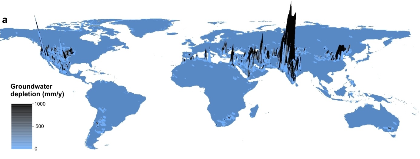
Fig. 2.23 A global map of groundwater depletion - peaks show areas where groundwater is most depleted.#
We can link the areas where groundwater is particularly depleted to areas where the groundwater footprint is particularly large relative to the size of the aquifer from which it is drawing water (Fig. 2.24).
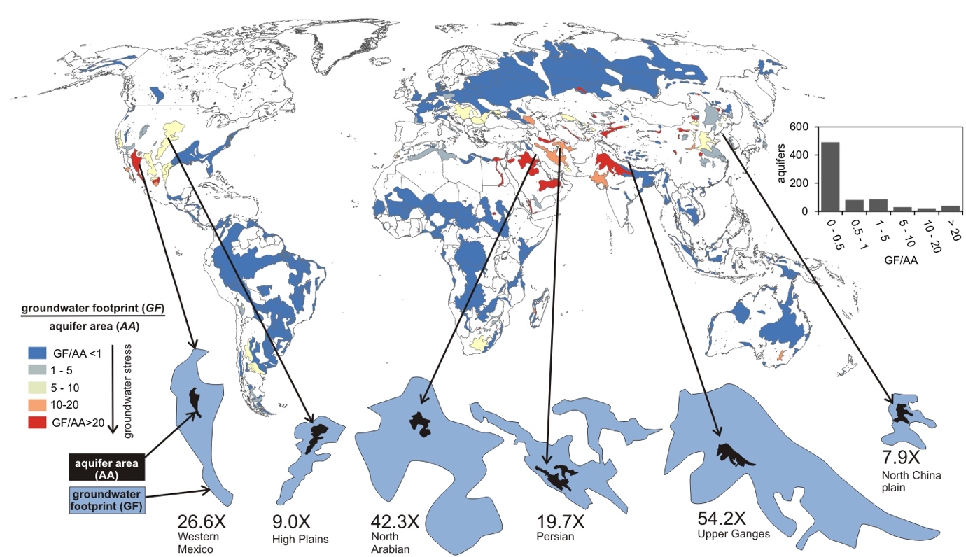
Fig. 2.24 Groundwater depletion is most severe where the ‘groundwater footprint’ is much larger than the underlying aquifer area.#
Another major challenge in groundwater systems is the transport of contaminants, that is something (potentially toxic) is released into the subsurface and travels with the groundwater, appearing in the water supply at some point later in time (depending on the hydraulic conductivity of the aquifer, and the hydraulic head difference driving the flow). In some respects we have learned the tools you would need to determine how long before a contaminant released into the groundwater would be seen at some point downstream. You could figure out the lines of equipotential, and the hydraulic conductivity, and then calculate the flow velocity, and this would yield time (with some knowledge of the distance travelled).
Control Volumes and Dispersion#
One way to think about this is using the ‘control volume’ and thinking that flow through advection moves the control volume along the X axis but flow through dispersion (molecular diffusion and mechanical or hydrodynamic dispersion) also moves the flow along in the Y and Z direction (Fig. 2.26).
A brief primer on diffusion
Diffusion is the spontaneous movement of particles from regions of high concentration to regions of low concentration. At the molecular level, this occurs due to random thermal motion of molecules. In groundwater, contaminants diffuse through pore water even in the absence of flow.
Diffusion is governed by Fick’s First Law, which states that the diffusive flux is proportional to the concentration gradient:
where \(J\) is the diffusive flux, \(D\) is the diffusion coefficient, and \(\frac{\partial C}{\partial x}\) is the concentration gradient. The negative sign indicates that diffusion occurs down the concentration gradient (from high to low concentration).
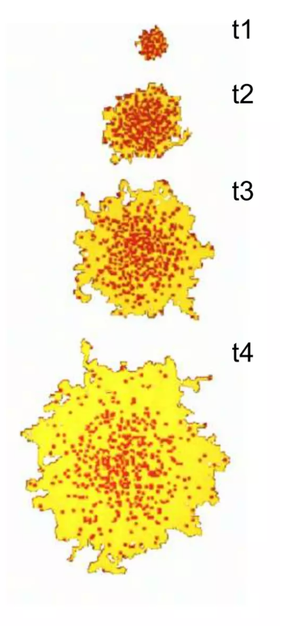
Fig. 2.25 Time series showing the spreading of dye through diffusion at four successive time steps, illustrating how concentration gradients diminish over time.#
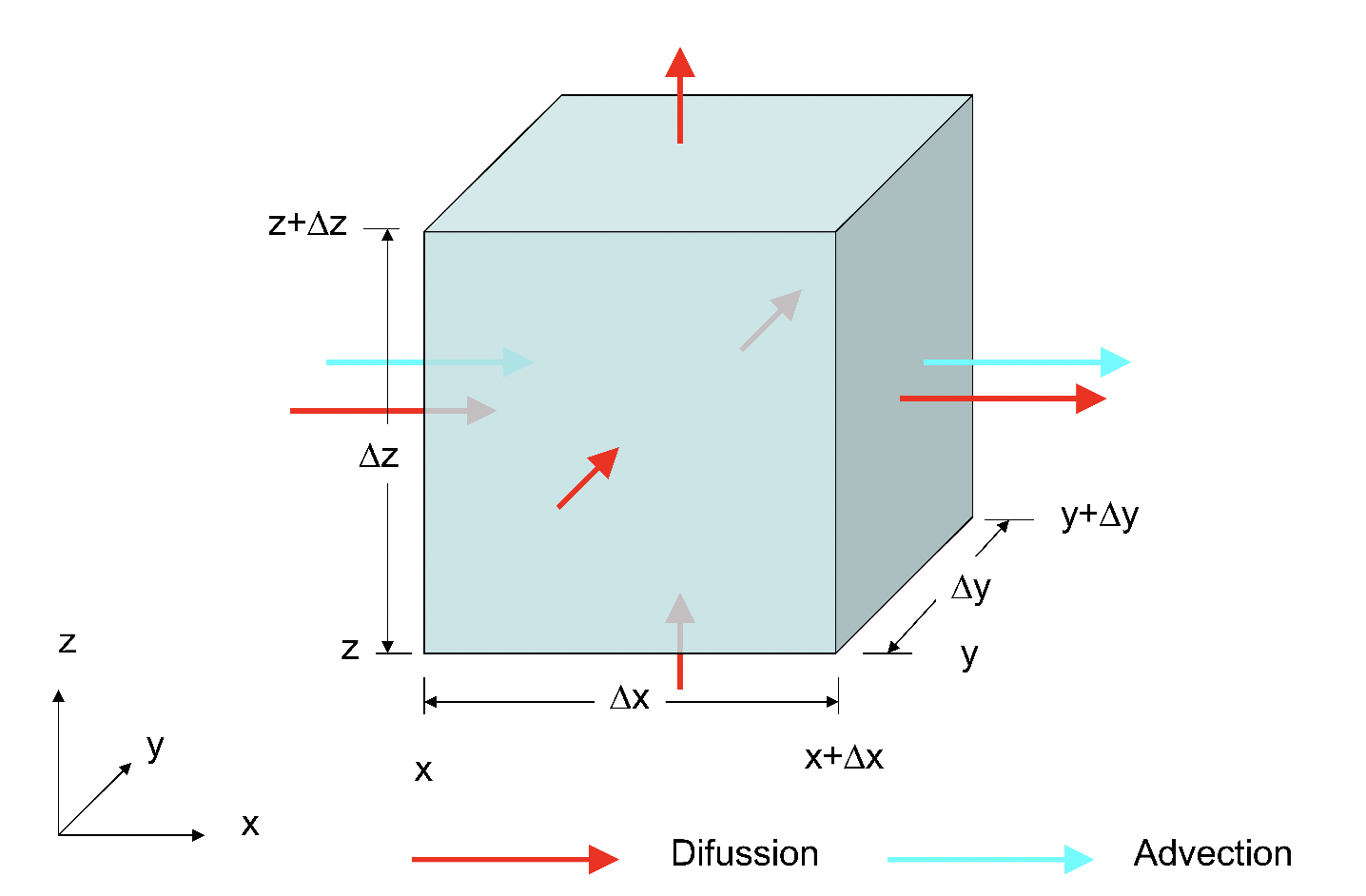
Fig. 2.26 A diagram showing how advection moves the control volume along the X axis while dispersion causes movement in the Y and Z directions.#
In beadpacks in the Institute for Energy and Environmental Flows you can see the stretching along the flowpath of an injection of dye (Fig. 2.27).
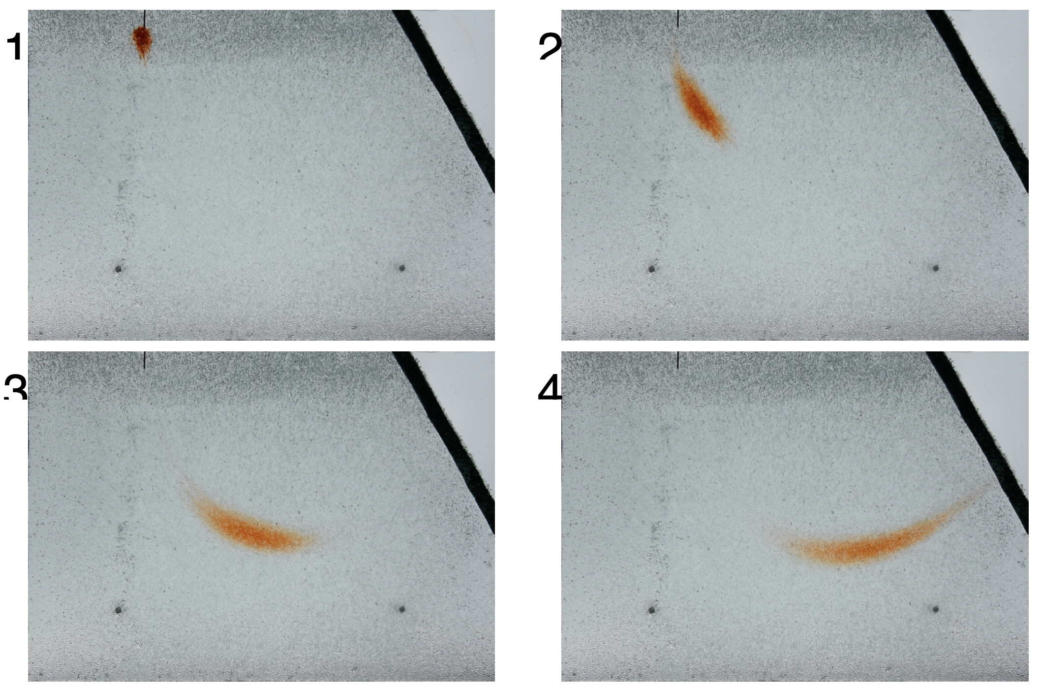
Fig. 2.27 Dye injection in a beadpack showing stretching along the flowpath.#
The Peclet Number#
Determining the relative importance of advection versus dispersion (so the growing shape of the contaminant plume during subsurface transport) is often done using the dimensionless Peclet Number (Fig. 2.28).
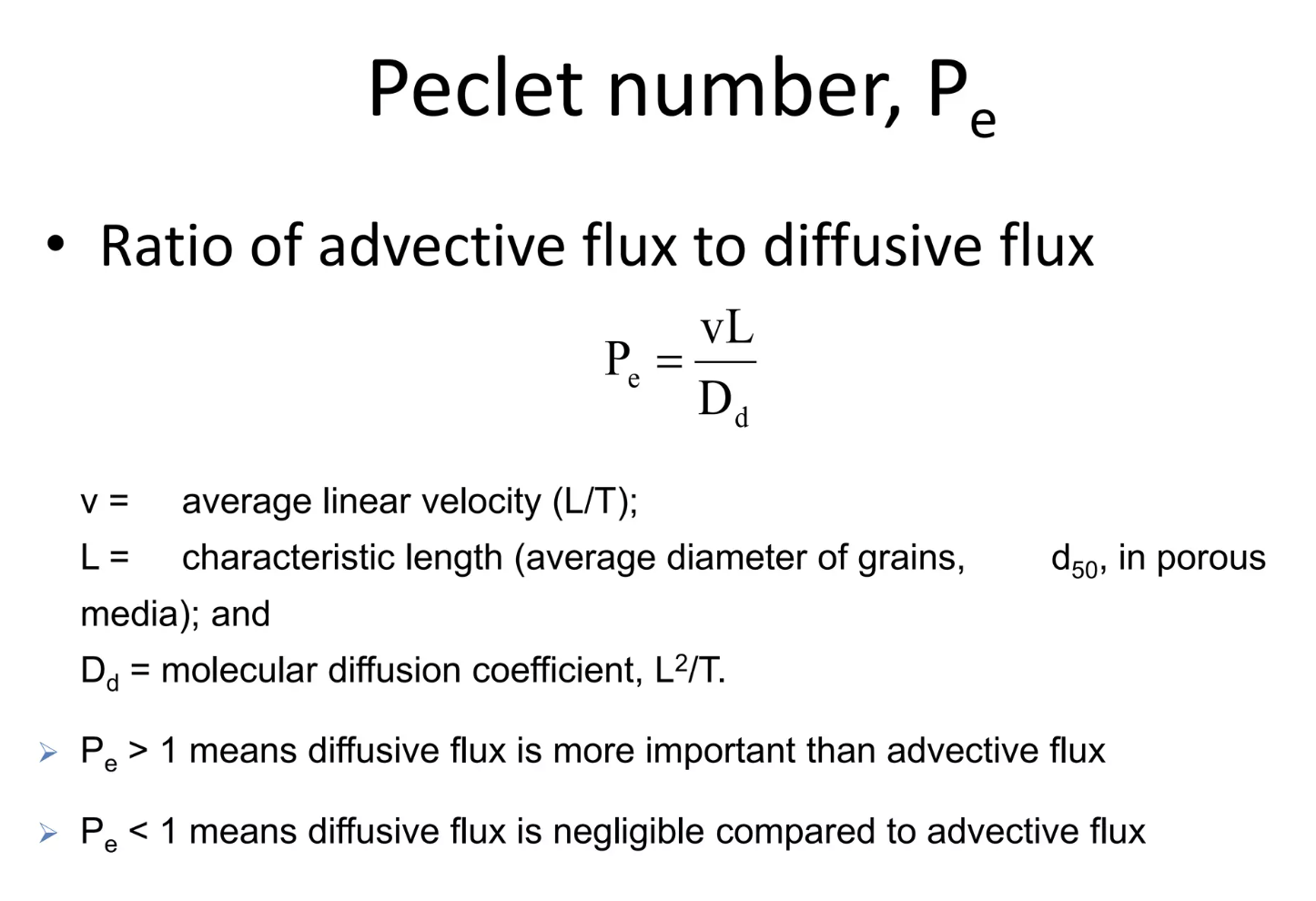
Fig. 2.28 The Peclet Number characterizes the relative importance of advection and dispersion in contaminant transport.#
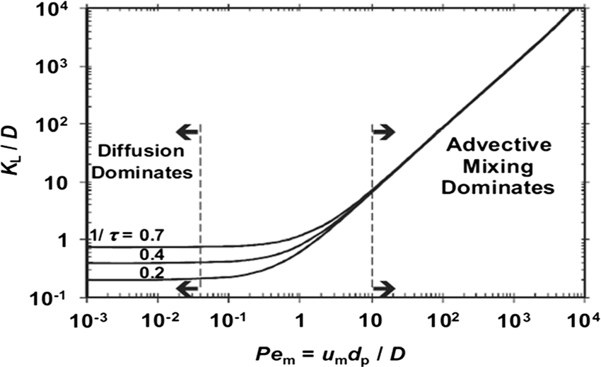
Fig. 2.29 Normalized dispersion coefficient plotted against Péclet number.#
Contaminant Plume Modeling#
If we assume that the contaminant spreads out in all directions as it moves along the flow of the groundwater, then we can track the shape of the contaminant plume away from the point source. Here the relative movement in the X direction versus the Y and Z direction is a function of the magnitude of the movement due to molecular diffusion versus that due to advective velocity and mechanical dispersion. With a series of simplifying assumptions (isotropic media, flow in the x direction etc.) we can use a gaussian model to track plume movement over time (Fig. 2.30).
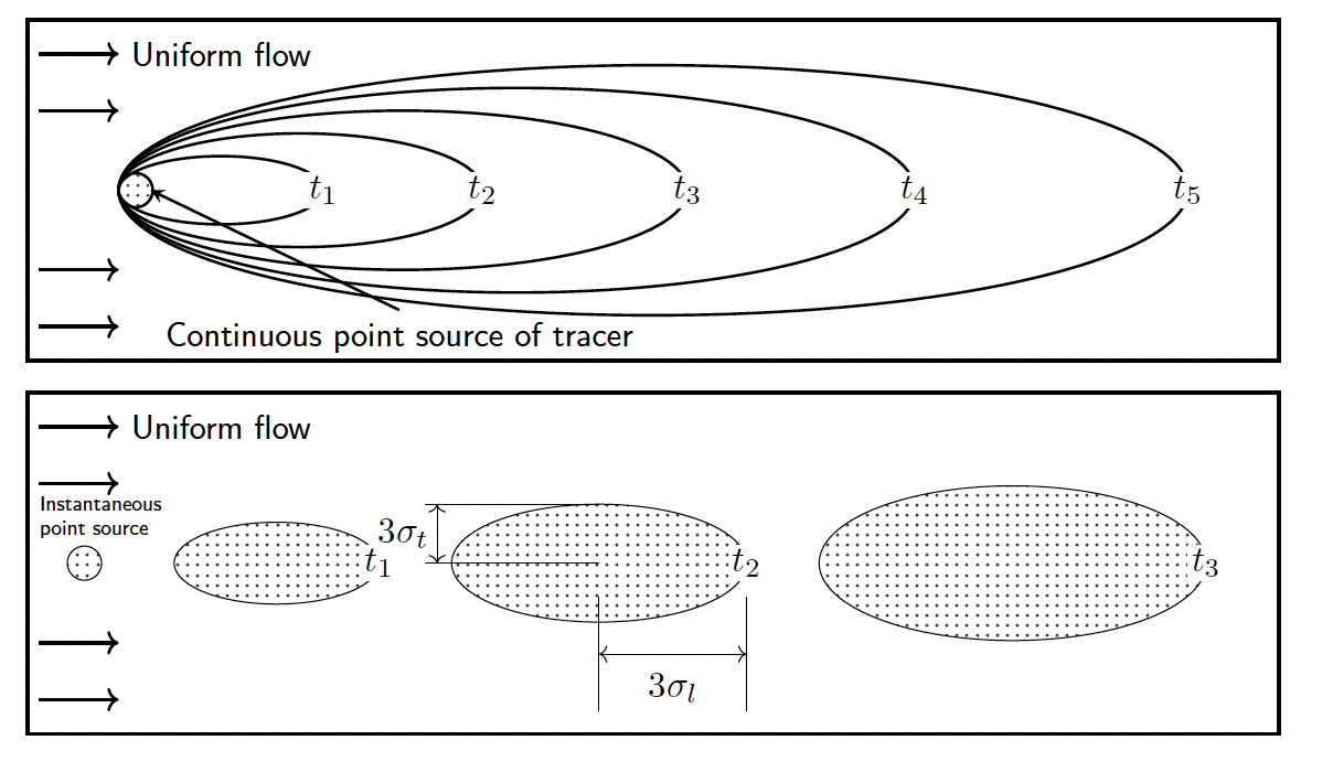
Fig. 2.30 Diagram showing the development of a contaminant plume in groundwater, tracking movement in three dimensions over time.#
This is similar to the maths behind following a plume of smoke in the atmosphere (Fig. 2.31, Fig. 2.32).

Fig. 2.31 A smoke plume in the atmosphere showing similar dispersion patterns.#
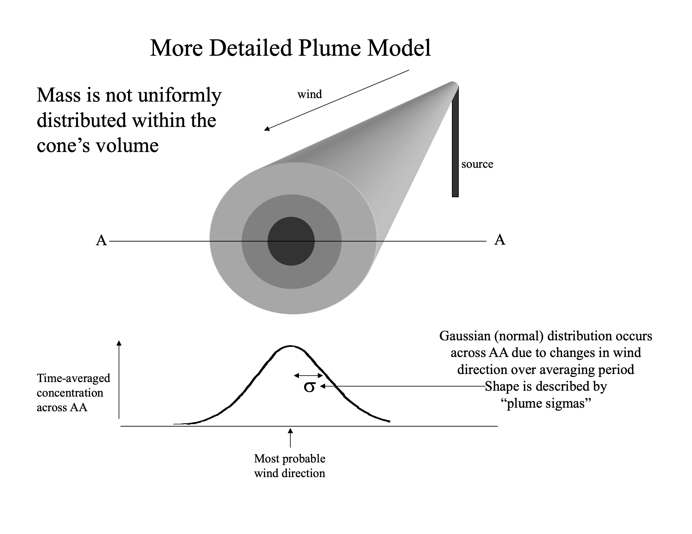
Fig. 2.32 Plume model diagram illustrating the mathematical framework for tracking dispersion.#
Contaminant Transport Models#
However, like most things, it is more complicated than this. The contaminant is not just subject to advection with the flow of the groundwater, but also diffusion (the process by which things move from high concentration to low concentration) and possibly chemical reaction with the porous media. This leads to an entirely different class of equations and models known as advective diffusive transport models. We wont go through the mathematics of these models but the standard formula is:
Where \(C\) is a contaminant, and I am curious how its concentration changes with time \(\left( \frac{\delta C}{\delta t} \right)\) and with distance \(\left( \frac{\delta C}{\delta x} \right)\). Because there are changes with time and with difference, we need to use a partial differential equation. In the partial differential equation above, \(D\) is the diffusion coefficient for the contaminant in water, \(v\) is the flow velocity \(\left( \frac{-K}{\rho} \dv{h}{x} \right)\) (can you figure out why this is the flow velocity from Darcy’s Law?), and \(R\) represents the chemical reactions that change the concentration with time. In the lecture we’ll talk through each of these terms, and how diffusion can be molecular diffusion or mechanical dispersion, and the types of chemical reactions that change the concentration of common contaminants.
Note
To explore the contamination of groundwater we are going to tell the story of arsenic poisoning in Bangladesh, why there are such high levels of arsenic in the groundwater and the various mechanisms that can help remedy this situation. This is just a specific example of an acute groundwater contamination problem and the way the community and scientists are trying to help remedy it. The details of this case study will be in the lecture slides.
Saline Intrusion#
Another major challenge in freshwater aquifers is the incursion of saline groundwater into the freshwater aquifer. Groundwater above the terrestrial (land) surface is recharged from rain, and is largely ‘fresh water’ and could be suitable for drinking. Groundwater beneath the ocean is salt water, and unless you undertake some serious desalination activities, is not suitable for drinking. At some point between the fresh subsurface groundwater and the salt subsurface groundwater, there is a mixing point where there is a freshwater-saltwater interface (Fig. 2.33 ).
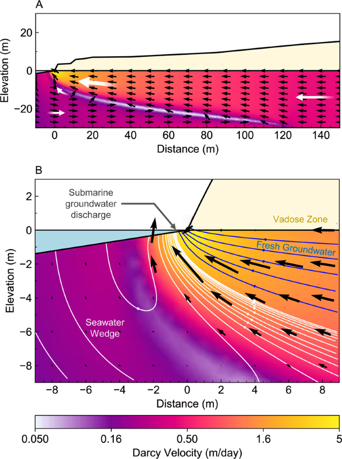
Fig. 2.33 An example of a freshwater-saltwater interface.#
Like all groundwater systems, the flow of groundwater goes from high hydraulic head to low hydraulic head. Every day – indeed twice a day – the tides move the envelope of seawater such that there is greater hydraulic head on the salt groundwater, pushing it further inland. When the tides move the envelope of water away from the coast, the freshwater will move back towards the ocean. Thus the freshwater-saltwater interface changes daily.
On top of this diurnal cycle, there are two larger scale things happening. One, sealevel is rising, due to the melting of ice and the thermal expansion of the ocean water. This increases the hydraulic head on the salt-groundwater, pushing it inland. Second, we have a large groundwater footprint and the fresh-groundwater near the coast are having water removed for agriculture and drinking and all the other things we said we need groundwater for in Lecture 4. This decreases the pressure in the coastal aquifers and drives more salt-groundwater inland (Fig. 2.34).
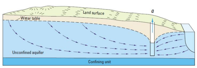
Fig. 2.34 Seawater can recharge an aquifer and contaminate it with salt water if we extract too much water near the coast. This problem will be exacerbated by sealevel rise, which will increase the hydraulic head on the saline side.#
We will finish the module with a consideration of sustainable groundwater resources and what does sustainable groundwater mean, practically, for all of us!