1.2. Energy and Carbon on the Planet

Key Concepts:

• Energy is received unevenly by Earth and redistributed via the movement of air and water.

• The uneven heating drives evaporation, condensation, and pressure differences in the atmosphere and at the atmosphere-ocean interface. These pressure difference lead to turbulent movement and eddies which are the workhorses of heat transport over the surface of the planet.

• The carbon cycle is made up of a series of reservoirs that contain carbon, and fluxes, which move carbon from one reservoir to another.

• The residence time of carbon in any one reservoir is calculated as the amount in that reservoir divided by the rate of input into that reservoir. It gives us a sense of how long a carbon atom might stay in any one reservoir before it moves to the next.

• Steady state is when the rate of input of carbon into a reservoir is the same as the rate of removal.

In this lecture we are going to consider where the energy driving Earth’s climate and environment comes from, and how it is redistributed around the planet. The energy ultimately comes from the sun, which delivers \(341.5 \ \mathrm{W m^{-2}}\) to the Earth. The way that our planet receives this energy, redistributes this energy, and the chemical, physical and biological reactions that harness or result from this energy drives all environmental and climate systems. Therefore, this is where it all begins. You will revisit these concepts later in the course, and during the lecture we will highlight where you will go through them again in more detail. When we work on these concepts then, we’ll delve more into the mathematics behind them. Here we will cover the broad topics more as an overview of the planetary system.

Earth doesn’t get all the power that the sun sends our way.

• Some is absorbed by gas in the atmosphere.

• Some bounces off clouds and returns to space through Rayleigh Scattering.

• Some is absorbed by clouds.

• Some bounces off the surface of the planet (particularly bright surfaces like snow).

About 46% is absorbed by the surface.

Our planet also re-radiates energy but this energy is at a longer wavelength than what we receive from the sun (Fig. 1.1).

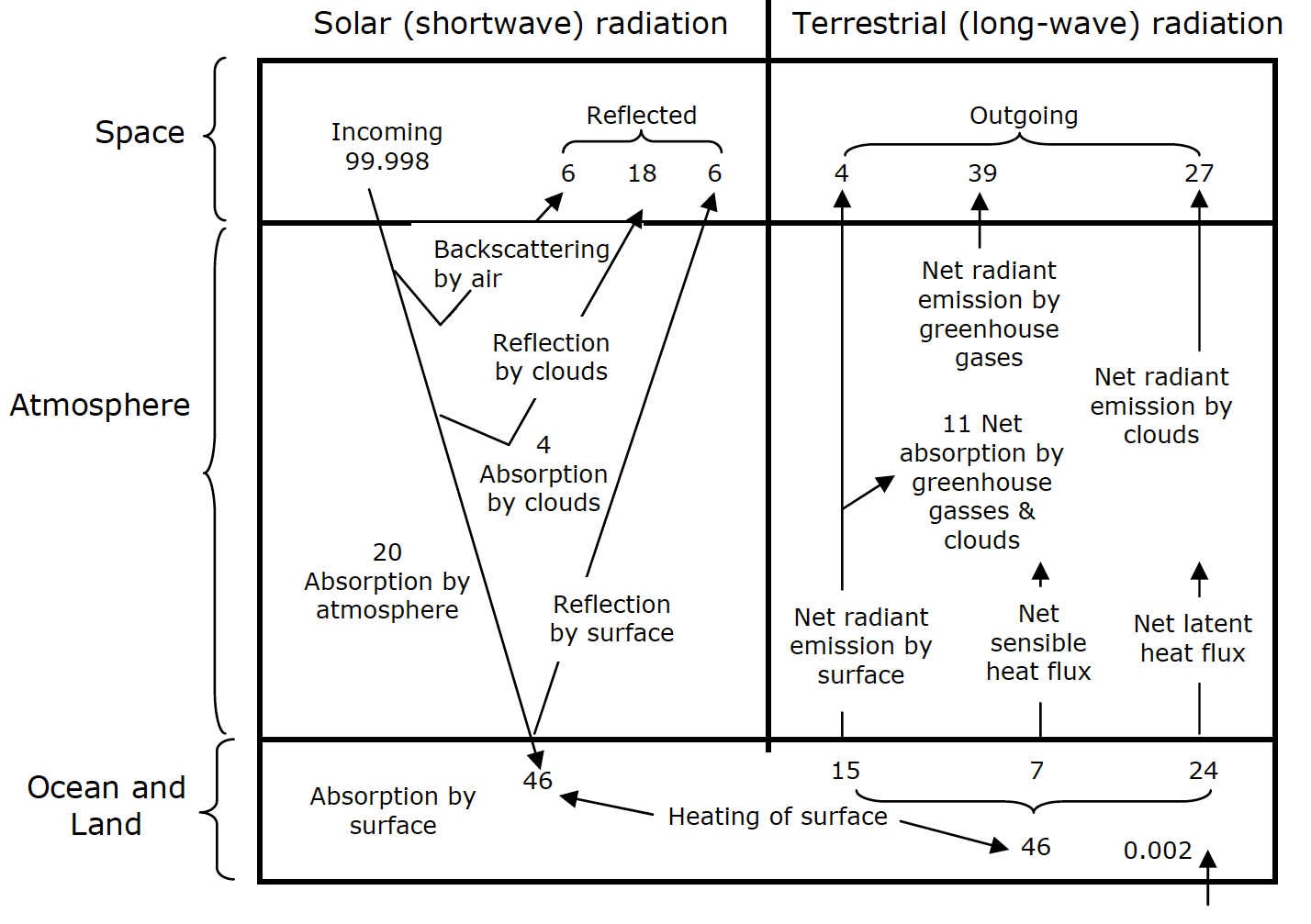
Fig. 1.1 A schematic of the earth’s energy cycle. Incoming solar radition is absorbed and reflected (left). The earth itself also emits longer wave radiation in the infra-red band (right).

What are each of these things happening on Earth’s surface? The heating of Earth’s surface drives physical changes which allows heat (in the form of radiation) to be released into the atmosphere.

For example, when water changes state from liquid to vapour during evaporation, this is called the latent heat flux, while when there is a temperature change at the surface but no change in state, this energy is released to the atmosphere as the sensible heat flux.

Different gases in our atmosphere are good at absorbing radiation or releasing radiation of different wavelengths. Fig. 1.2 shows the wavelengths of the downward transmission of solar radiation and the upgoing longwave radiation. Gases in our atmosphere both absorb wavelengths of radiation that are short (as in those coming from the sun) and long (as those emitted from the Earth). Different gases behave differently, and later this term you will learn what in the physics of the molecule makes a good greenhouse gas.

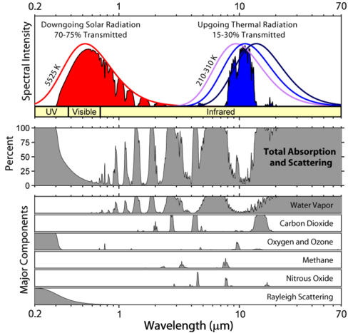
Fig. 1.2 The raditation transmitted and absorbed by the atmosphere.

The balance of energy coming in from the sun and then interacting with the surface of the planet, causing both changes of state and changes in local temperature, and the transmission of this energy through the atmosphere, this drives the hydrological cycle, the movement of heat, air, water, and the carbon in that air and water. What the Earth does with the energy it receives, and the impact that this has on the climate system, is the focus of this course.

The sun doesn’t heat the Earth’s surface evenly, but the re-radiation of energy from Earth’ surface is more even. This leads to global energy imbalance that drives the transfer of water and air (Fig. 1.3).

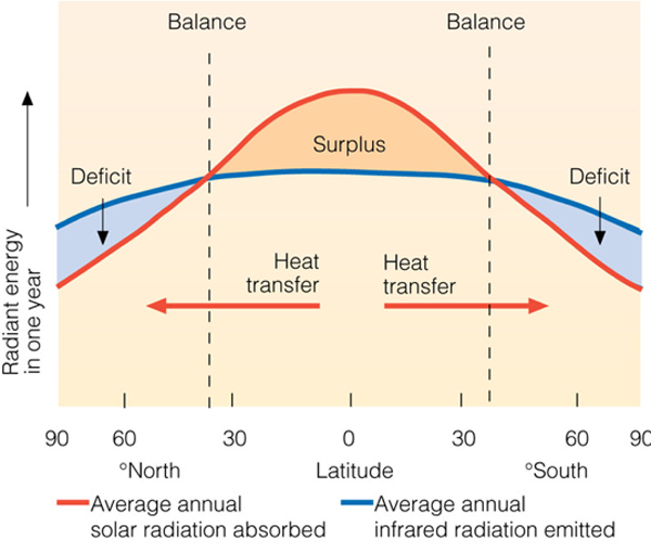
Fig. 1.3 The balance of incoming and outgoing radiation plotted against latitude. The surplus of radiation at the lower latitudes is transported north and south to higher latitudes.

The heat is transferred when warm air rises and moves towards colder regions, and when warm water is moved in the oceans from the tropics (warm) to the poles (cold). We can quantify the energy transfer and parse it into which fraction is transported by the air and which is transported by the water (Fig. 1.4).

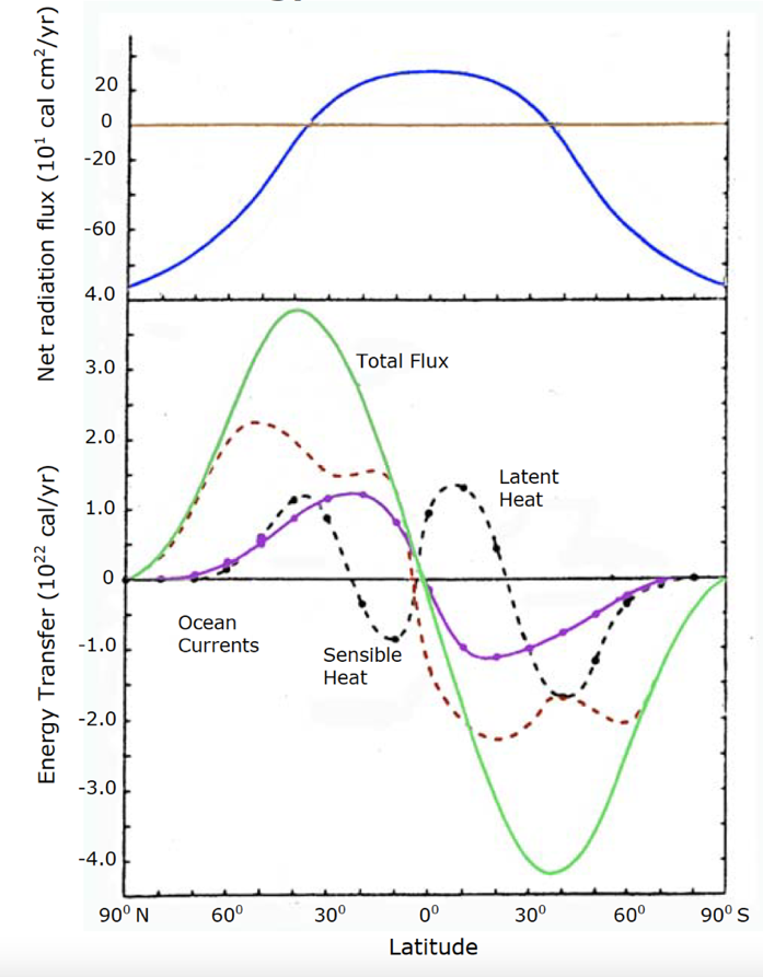
Fig. 1.4 How is energy redistributed from the equator to the poles? It is carried by both the atmosphere and the oceans. This energy redistribution results from temperature gradients. Therefore, it is key for all environmental systems.

We know instinctively that heat is redistributed because we, in Cambridge, have much warmer temperatures than we would have if heat wasn’t transported from the equator to the poles. In Fig. 1.5, you can see the equilibrium temperature as a function of latitude with the latitude of Cambridge noted on the diagram. As you can see, Cambridge is much warmer (over 20 DegC warmer!) than it would be if there were no heat transport over the planet.

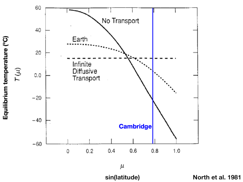
Fig. 1.5 Camrbidge is warmer than it should be.

How is this heat actually transported? It is transported in part because of movement in the oceans and in part because of movement in the atmosphere. There are large scale circulation patterns (‘eddies’) that are established in the ocean and atmosphere, due to the creation of pressure differences due to differential heating leading to evaporation and condensation. This movement of heat and water vapour on the rotating planet sets up circulation cells in the atmosphere and circulation patterns in the oceans (Fig. 1.6). In our lectures on the Global Environment we’ll discuss these broad patterns of movement.

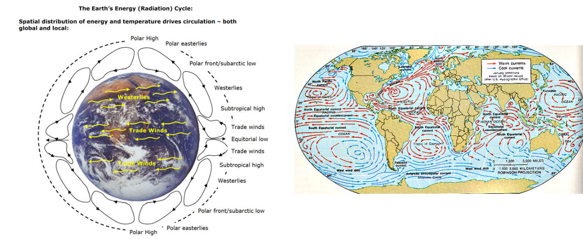
Fig. 1.6 Movement in the atmosphere (left) and oceans (right).

You have likely heard that Cambridge is warm because of the transfer of heat by the Gulf Stream, the deep western boundary current that brings warm water from the Caribbean to the North Atlantic. In the ocean, large-scale mean currents, including western boundary currents, are largely responsible for transporting heat from the tropics towards the poles. However, in the atmosphere, the physical workhorse for the movement of heat around the planet are eddies (including the storm systems that control our weather). Eddies, which occur in both the ocean and atmosphere, are circular motions of air and water (Fig. 1.7). Eddies more broadly occur during turbulent flow and refer generally to the movement of fluid in a direction counter to that of the general flow. We’ll discuss more about the turbulent flow in Lecture 5.

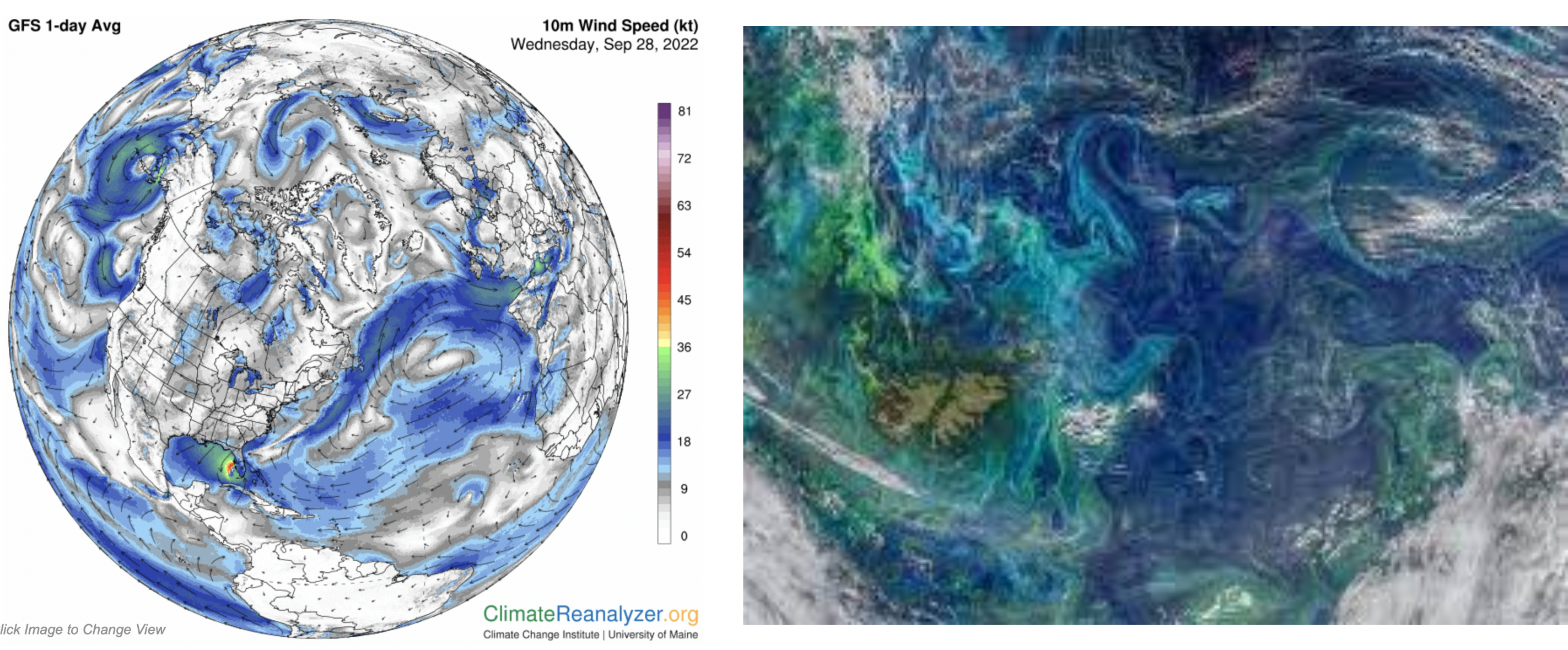
Fig. 1.7 Eddies in the atmosphere (storms, left) and the ocean (right).

The Carbon Cycle

Residence time, Reservoirs, Fluxes, and Steady State

The carbon cycle refers to the movement, or exchange, of carbon around the planet through various reservoirs. Carbon is important as a gas because in its oxidized form (\(\mathrm{CO_2}\)) and in its reduced form (\(\mathrm{CH_4}\)), it is the strongest greenhouse gas in our atmosphere, keeping the planet warm. Carbon is important dissolved in liquid (as \(\mathrm{H_2CO_3}\), \(\mathrm{HCO_3^-}\), and as \(\mathrm{CO_3^{2-}}\)) because it acts as a pH buffer and allows the oceans to maintain equable pH. Carbon is also the backbone of life on our planet.

Reservoirs of carbon at Earth’s surface are pools or environments that can be uniquely defined. Common units are grams (\(\mathrm{g}\)), parts-per-million-volume (\(\mathrm{ppmv}\)), moles (\(\mathrm{mol}\)), or moles-per-liter (also called Molar) (\(\mathrm{mol \ L^{-1}}\) or \(\mathrm{M}\)).

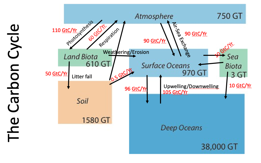
Fig. 1.8 The carbon cycle on earth, showing the major stores of carbon, their capacities, residence times, and the fluxes between them. Units are Gigatonnes (GT) of Carbon per year (\(1 GT = 10^{15} g\)).

Fluxes of carbon are the rate of exchange between one reservoir and another reservoir. Units are amount-per-time, in this case Gigatonnes (GT) of Carbon per year (\(1 GT = 10^{15} g\)).

The schematic of the global carbon cycle in carbon_cycle only shows the reservoirs at Earth’s surface. Over longer time periods there is a much slower exchange of carbon between these reservoirs and rocks and the deep Earth below. That is less important for this course, where we are concerned with surface environments.

Looking at various reservoirs in this way allows us to consider the concept of Residence Time. Residence time refers to the average amount of time that carbon spends in any one of the reservoirs before it moves to the next reservoir. We can calculate this by knowing the amount in the reservoir (total number of moles, or grams) and dividing it by the rate that it is taken from or added to the reservoir (in moles or grams per time). This gives us a rough idea of how long carbon might stick around in any one reservoir.

Box models like the ones shown schematically in carbon_cycle for the carbon cycle above will come up many times throughout this course, and this week’s supervision sheet will cover the mathematics behind box models. At its most basic, if we think about the quantity of something in a reservoir, in this case the amount of carbon in one of our carbon cycle reservoirs, then if the rate at which it is being added (amount-per-time) equals the rate at which it is being taken away (amount-per-time), the concentration in the reservoir won’t change. We call this Steady State.. If the amount being put in is larger than the amount being taken out, then the concentration will rise and if the amount being taken out is larger than the amount being put in, then the concentration will fall.

In the real world, the rate that carbon is removed from a reservoir is proportional to the amount that is in that reservoir. We can think about this practically if we consider real processes. If I add carbon to the atmosphere, then the concentration of carbon as gas in the atmosphere will increase. But this increase will cause the chemical and physical reactions that remove carbon from the atmosphere to also increase. This can be for direct reasons or indirect reasons. For example:

• Chemical reactions that consume carbon gas in the atmosphere (say the oxidation of methane will \(\mathrm{OH}\) radicals) will accelerate when there is more reactant (via Le Chatelier’s principle)

• Physical reactions that remove gas, like the dissolution of carbon dioxide into the ocean that scales with wind speed, will each remove more carbon dioxide when they happen.

• Indirectly, increased carbon in the atmosphere increases temperature, and this can accelerate things like photosynthesis and other temperature-dependent reactions.

What this means practically is that at long enough timescales, most systems will trend towards steady state, where the inputs and outpus are balanced – that is if there is a change in the inputs, the outputs will adjust to match the inputs.

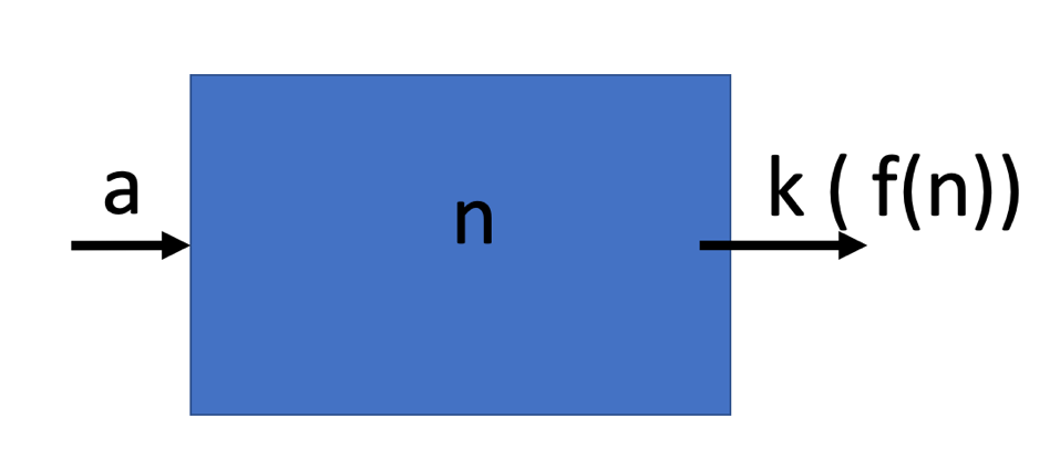
Fig. 1.9 A schematic of a basic box model, with a flux \(a\) in, and a flux out that is a function of the amount \(n\) in the box, \(k n\).

box_model shows a conceptual box model for some species \(n\) which is being supplied to the box by the input flux \(a\), and removed from the box by a removal process that is a function of the amount of \(n\) in the box, \(k(n)\).

We can write a simple equation that allows us to model how the concentration of \(n\) will change in the box over time (\(t\)).

Units!

\[\begin{split} n &= \mathrm{concentration} \\ t &= \mathrm{time} \\ a &= \mathrm{concentration~time^{-1}} \\ k &= \mathrm{time^{-1}} \end{split}\]

(1.1)\[\dv{n}{t} = a - k n\]

In your supervision you will cover how we solve this type of differential equation, and you will get the opportunity to work on these in the supervision sheet. The solution for \(n\) as a function of time is:

(1.2)\[n(t) = \frac{a}{k} - \left[ \frac{a}{k} - n_{o} \right] e^{-kt}\]

We can think about the functional form that this equation takes. At long timescales, the second term drops out and the amount of \(n\) in the box becomes \(\frac{a}{k}\). However, when you perturb the system (increase or decrease the input, \(a\), or change the rate constant for the removal, \(k\)) the system approaches a new concentration, \(\frac{a}{k}\).

Consider the application of this sort of a model for the atmosphere (the reservoir) and for carbon dioxide (co2_atm) and methane (ch4_atm).

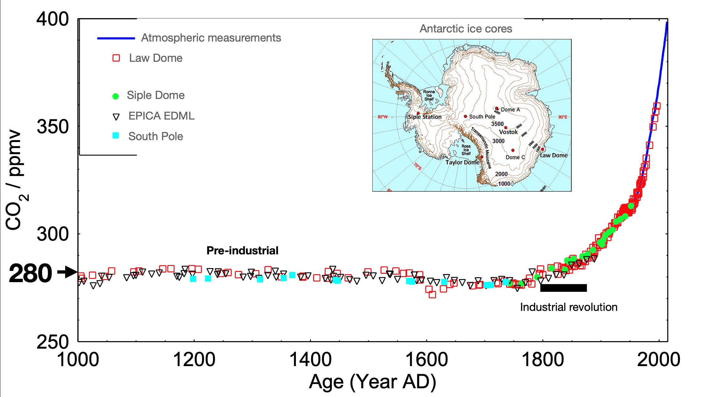
Fig. 1.10 A plot showing the change in atmospheric \(\mathrm{CO_2 \ ppmv}\) over the last \(\mathrm{1000 \ years}\). Inset, a map of Antarctica showing the locations where ice cores were taken.

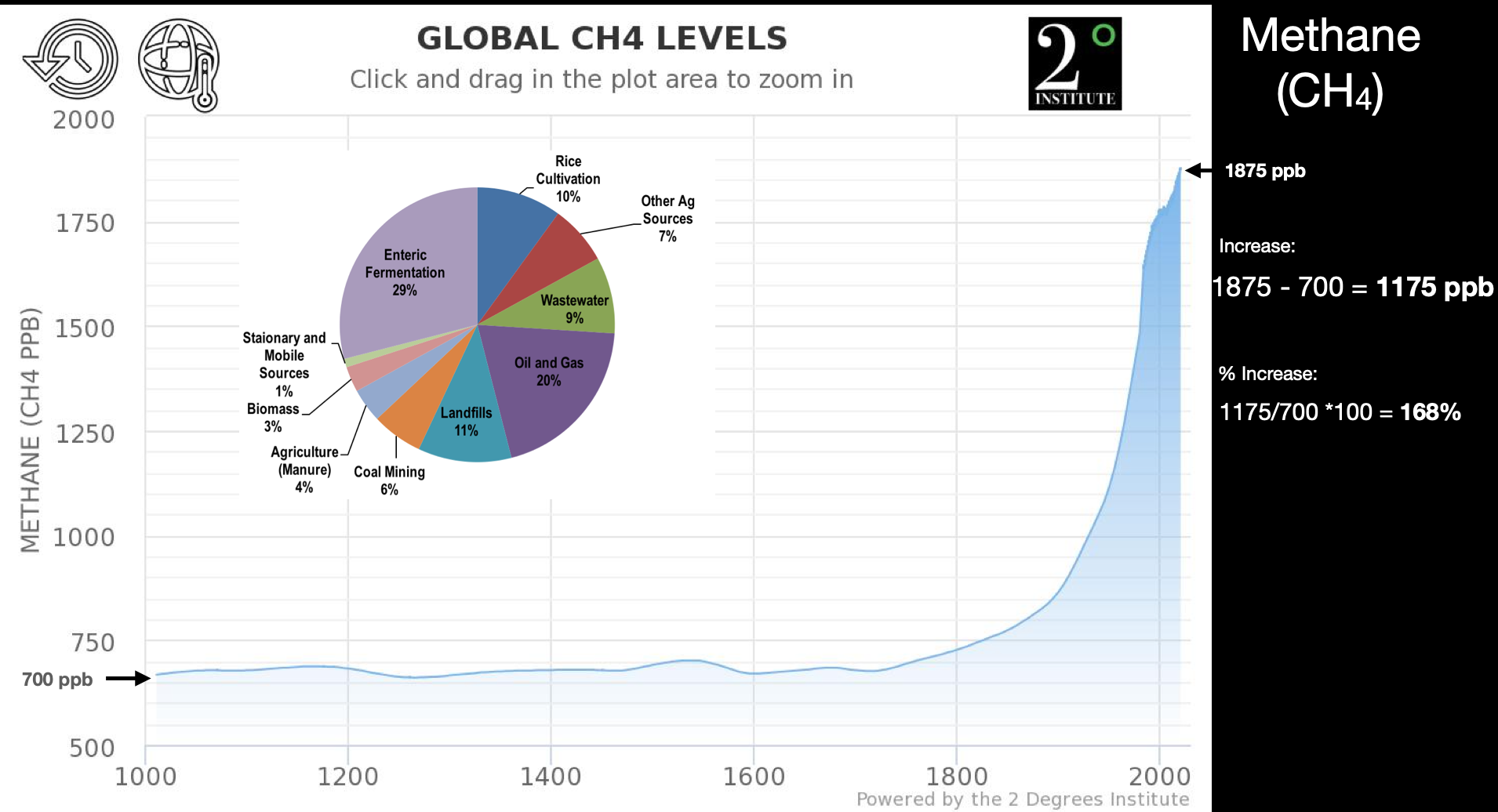
Fig. 1.11 Global atmospheric methane levels in \(\mathrm{ppb}\) over the last 1000 years. Inset, pie chart showing the contribution to the atmospheric methane flux of various sources.

In each case there are sources of carbon dioxide (co2_atm) and methane (ch4_atm) that are exceeding the sinks, and the concentration is increasing. If the sources were to decrease, what would happen to the concentrations? They would decrease, and how quickly they would decrease would depend on the residence time of these elements in the atmosphere (which relates to how much is there and the rate of addition and removal).

Where will you see this elsewhere in the course? Box models and the mathematics behind box models will come up again and again throughout the course! It is a good idea to spend time with your supervisors to make sure you are comfortable with the functional form of the equation that describes the time evolution of something in a box. In this lecture it was carbon, but later this week it will refer to the storage of water in a groundwater aquifer,

the mass balance of ice sheets,

and the volume of water in reservoirs needed to prevent flooding.

Next term we will revisit this in the form of the ocean carbon cycle and how the ocean sequesters carbon at depth.

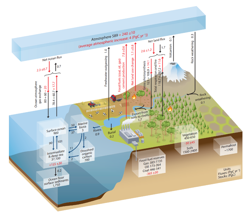
Fig. 1.12 An illustration of the various fluxes in the carbon cycle, designed by the IPCC.