1.3. The Carbon Cycle#
Residence time, Reservoirs, Fluxes, and Steady State
The carbon cycle refers to the movement, or exchange, of carbon around the planet through various reservoirs. Carbon is important as a gas because in its oxidized form (\(\mathrm{CO_2}\)) and in its reduced form (\(\mathrm{CH_4}\)), it is the strongest greenhouse gas in our atmosphere, keeping the planet warm. Carbon is important dissolved in liquid (as \(\mathrm{H_2CO_3}\), \(\mathrm{HCO_3^-}\), and as \(\mathrm{CO_3^{2-}}\)) because it acts as a pH buffer and allows the oceans to maintain equable pH. Carbon is also the backbone of life on our planet.
Reservoirs of carbon at Earth’s surface are pools or environments that can be uniquely defined. Common units are grams (\(\mathrm{g}\)), parts-per-million-volume (\(\mathrm{ppmv}\)), moles (\(\mathrm{mol}\)), or moles-per-liter (also called Molar) (\(\mathrm{mol \ L^{-1}}\) or \(\mathrm{M}\)).
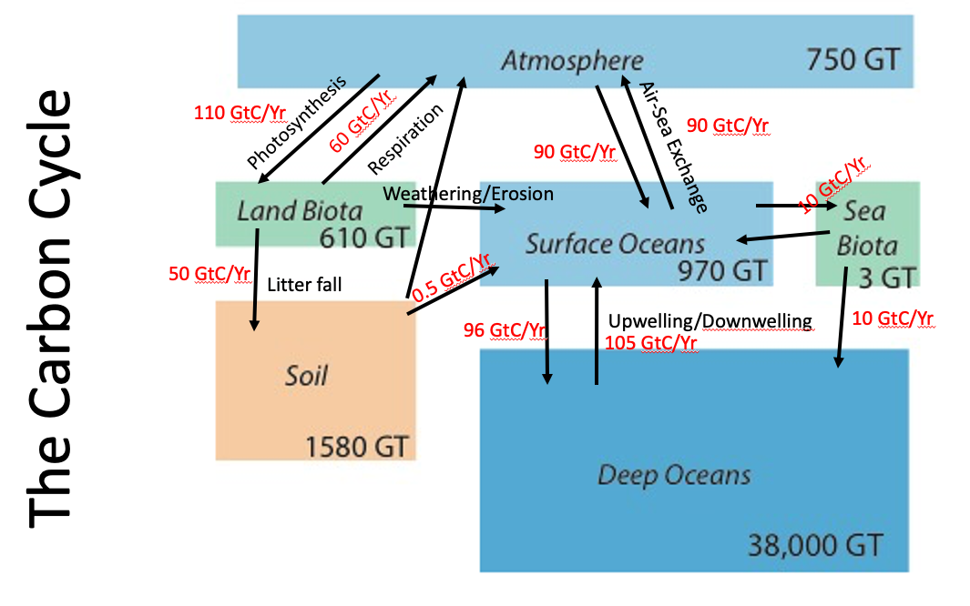
Fig. 1.8 The carbon cycle on earth, showing the major stores of carbon, their capacities, residence times, and the fluxes between them. Units are Gigatonnes (GT) of Carbon per year (\(1 GT = 10^{15} g\)).#
Fluxes of carbon are the rate of exchange between one reservoir and another reservoir. Units are amount-per-time, in this case Gigatonnes (GT) of Carbon per year (\(1 GT = 10^{15} g\)).
The schematic of the global carbon cycle in Fig. 1.8 only shows the reservoirs at Earth’s surface. Over longer time periods there is a much slower exchange of carbon between these reservoirs and rocks and the deep Earth below. That is less important for this course, where we are concerned with surface environments.
Looking at various reservoirs in this way allows us to consider the concept of Residence Time. Residence time refers to the average amount of time that carbon spends in any one of the reservoirs before it moves to the next reservoir. We can calculate this by knowing the amount in the reservoir (total number of moles, or grams) and dividing it by the rate that it is taken from or added to the reservoir (in moles or grams per time). This gives us a rough idea of how long carbon might stick around in any one reservoir.
Box models like the ones shown schematically in Fig. 1.8 for the carbon cycle above will come up many times throughout this course, and this week’s supervision sheet will cover the mathematics behind box models. At its most basic, if we think about the quantity of something in a reservoir, in this case the amount of carbon in one of our carbon cycle reservoirs, then if the rate at which it is being added (amount-per-time) equals the rate at which it is being taken away (amount-per-time), the concentration in the reservoir won’t change. We call this steady state. If the amount being put in is larger than the amount being taken out, then the concentration will rise and if the amount being taken out is larger than the amount being put in, then the concentration will fall.
In the real world, the rate that carbon is removed from a reservoir is proportional to the amount that is in that reservoir. We can think about this practically if we consider real processes. If I add carbon to the atmosphere, then the concentration of carbon as gas in the atmosphere will increase. But this increase will cause the chemical and physical reactions that remove carbon from the atmosphere to also increase. This can be for direct reasons or indirect reasons. For example:
Chemical reactions that consume carbon gas in the atmosphere (say the oxidation of methane will \(\mathrm{OH}\) radicals) will accelerate when there is more reactant (via Le Chatelier’s principle)
Physical reactions that remove gas, like the dissolution of carbon dioxide into the ocean that scales with wind speed, will each remove more carbon dioxide when they happen.
Indirectly, increased carbon in the atmosphere increases temperature, and this can accelerate things like photosynthesis and other temperature-dependent reactions.
What this means practically is that at long enough timescales, most systems will trend towards steady state – that is if there is a change in the inputs, the outputs will adjust to match the inputs.
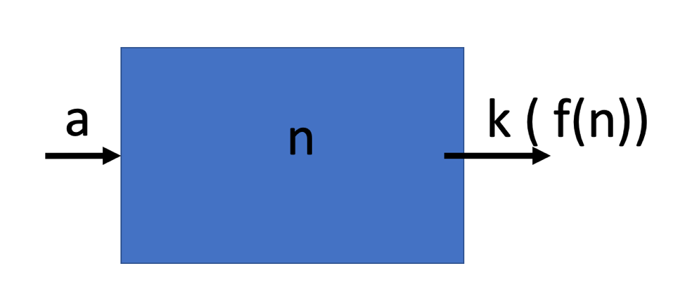
Fig. 1.9 A schematic of a basic box model, with a flux \(a\) in, and a flux out that is a function of the amount \(n\) in the box, \(k n\).#
Fig. 1.9 shows a conceptual box model for some species \(n\) which is being supplied to the box by the input flux \(a\), and removed from the box by a removal process that is a function of the amount of \(n\) in the box, \(k(n)\).
We can write a simple equation that allows us to model how the concentration of \(n\) will change in the box over time (\(t\)).
In the lecture we will cover different ways to deal with this sort of equation, and you will get the opportunity to work on these in the supervision sheet. The solution for \(n\) as a function of time is:
We can think about the functional form that this equation takes. At long timescales, the second term drops out and the amount of \(n\) in the box becomes \(\frac{a}{k}\). However, when you perturb the system (increase the input, \(a\), or change the rate constant for the removal, \(k\)) the system approaches a new concentration, \(\frac{a}{k}\).
We can consider this in terms of carbon dioxide (Fig. 1.10) and methane (Fig. 1.11) in the atmosphere.
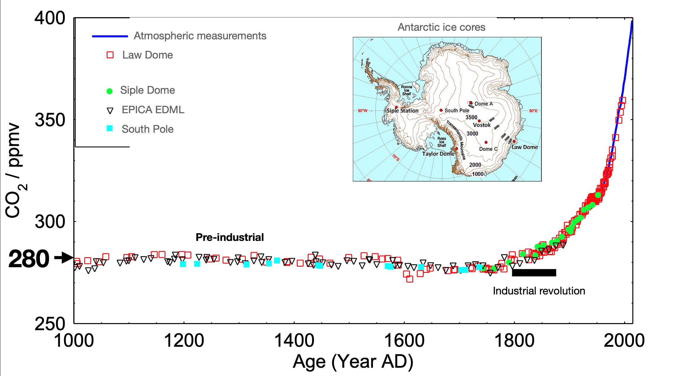
Fig. 1.10 A plot showing the change in atmospheric \(\mathrm{CO_2 \ ppmv}\) over the last \(\mathrm{1000 \ years}\). Inset, a map of Antarctica showing the locations where ice cores were taken.#
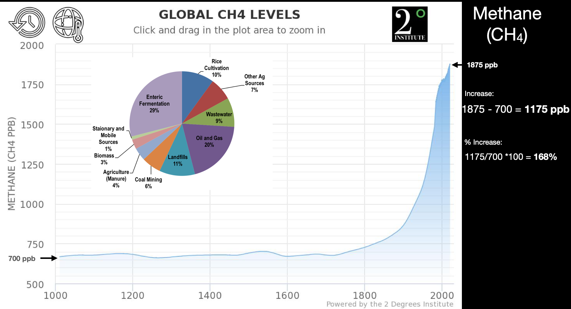
Fig. 1.11 Global atmospheric methane levels in \(\mathrm{ppb}\) over the last 1000 years. Inset, pie chart showing the contribution to the atmospheric methane flux of various sources.#
Where will you see this elsewhere in the course? Box models and the mathematics behind box models will come up again and again throughout the course! It is a good idea to spend time with your supervisors to make sure you are comfortable with the functional form of the equation that describes the time evolution of something in a box. In this lecture it was carbon, but later this term it will refer to the storage of water in a groundwater aquifer,
the mass balance of ice sheets,
and the volume of water in reservoirs needed to prevent flooding.
Next term we will revisit this in the form of the ocean carbon cycle and how the ocean sequesters carbon at depth.
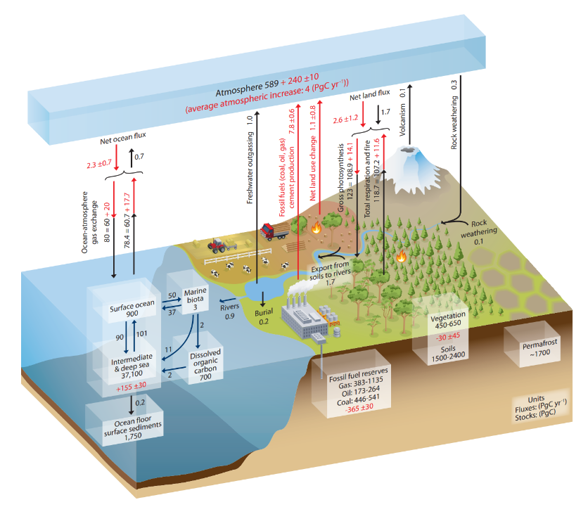
Fig. 1.12 An illustration of the various fluxes in the carbon cycle, designed by the IPCC.#