6.4. Structure and mean circulation of the atmosphere#
In the next three lectures, we will discuss the mean (time and longitudinally-averaged) structure of the atmosphere as a function of height and latitude. We will discuss the implications for this structure on the mean wind in geostrophic balance. We will also discuss the processes that lead to poleward heat transport and will introduce a few simple models to estimate the global heat distribution that results from a balance between net radiation and transport processes.
Fig. 6.3 showed the mean distribution of temperature in the atmosphere as a function of height and latitude. The north/south gradients in temperature are related to the wind speed through geostrophic and hydrostatic balance. Recall that geostrophic balance (Eq. (6.7)) relates the velocity vector with gradients in pressure. Here, we are considering the velocity associated with the mean (time and longitudinally-averaged) temperature and pressure. Therefore \(p=p(y,z)\) and \(\partial p/\partial x=0\) and from Eq. (6.7), the north/south component of the geostrophic wind will be zero \((v=0)\).
The \(x\)-component of the geostrophic wind satisfies
Notice that we have used a partial derivative on the RHS since \(p\) also varies in \(z\). We will also assume that the pressure is in hydrostatic balance:
From the ideal gas law
where \(M\) is the mean molar mass of air and \(R\) is the ideal gas constant. Using Eq. (6.13) in Eqns. (6.11) and (6.12) gives
and
where the last relation in each equation follows from the differentiation rule for the natural logarithm. We can eliminate the pressure and combine these two equations by cross-differentiating these equations. Taking the derivative of Eq. (6.14) with respect to \(z\),
and taking the derivative of Eq. (6.15) with respect to \(y\) gives
Since the RHS of these equations are identical, it follows that
Applying both derivatives using the product and reciprocal rules and re-arranging gives a relationship between the vertical derivative of the wind speed and the temperature gradient:
This equation is called thermal wind balance and we refer to \(u\) as the thermal wind. In practice, the second term on the RHS of Eq. (6.16) is usually smaller than the first, and the thermal wind approximately satisfies
The thermal wind can be found by integrating the thermal wind balance equation with respect to \(z\) and fixing the thermal wind at a reference level to determine the constant of integration. We often do this by setting \(u=0\) at the ground (\(z=0\)).
Returning to Fig. 6.3, in the Northern Hemisphere, \(\partial T/\partial y<0\) (temperature decreases in the northwards direction). Recall that \(f\) is related to the Earth’s angular velocity vector projected onto the local vertical direction and in the Northern Hemisphere, \(f>0\). Hence, with \(u=0\) at \(z=0\), we expect the thermal wind to have \(u>0\). In the Southern Hemisphere \(\partial T/\partial y < 0\), but since \(f<0\) we again have \(u>0\).
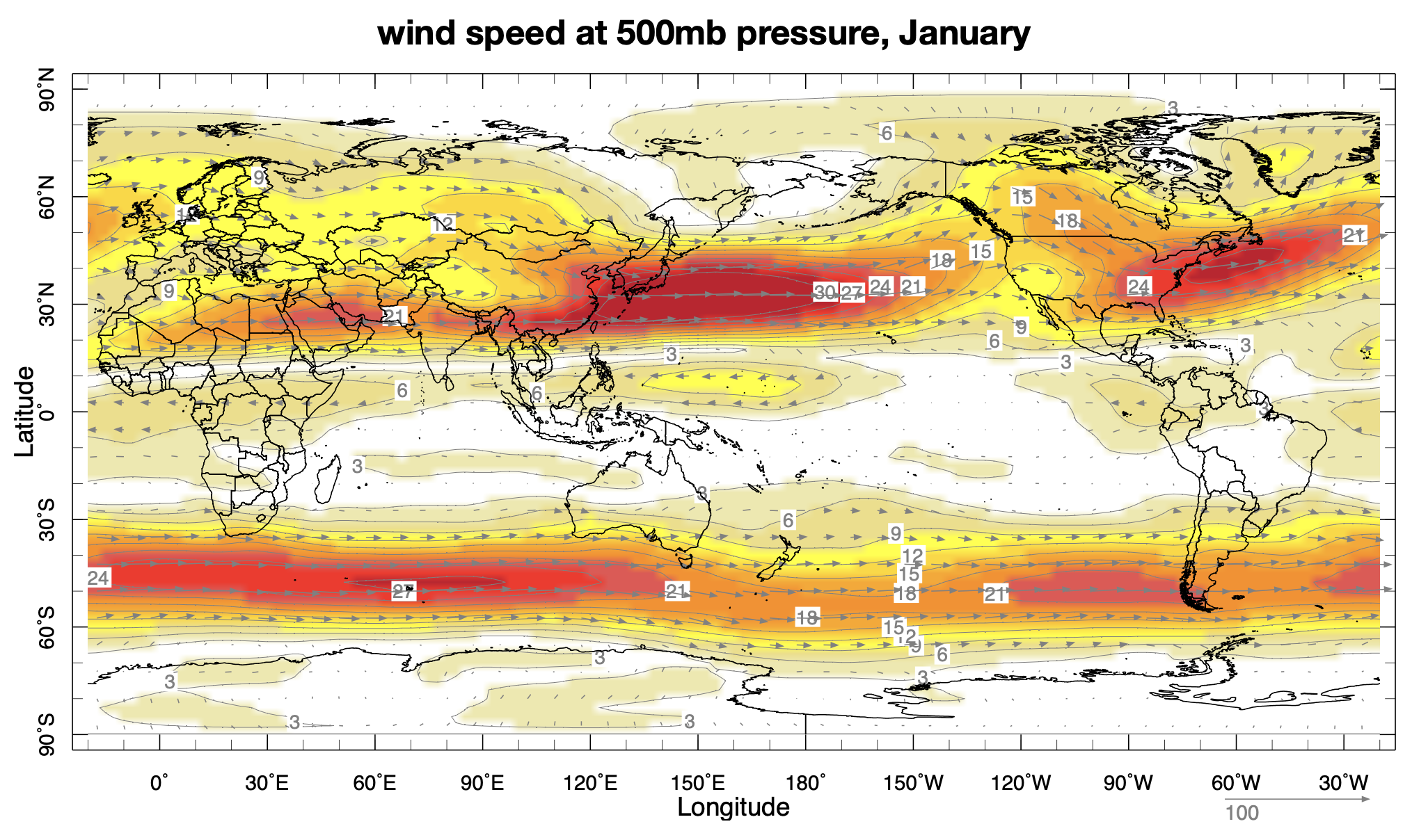
Fig. 6.14 Climatological (time-averaged) wind speed speed (m/s) for January.#
Fig. 6.14 shows the average (climatological) wind speed for January. The highest wind speeds are associated with mid-latitude jets of wind circling the globe and blowing from west to east. These ‘westerly jets’ are approximately in thermal wind balance. Note that the maximum wind speed is usually found between 30N and 60N where the mean north/south temperature gradient is large (compare with Fig. 6.3).
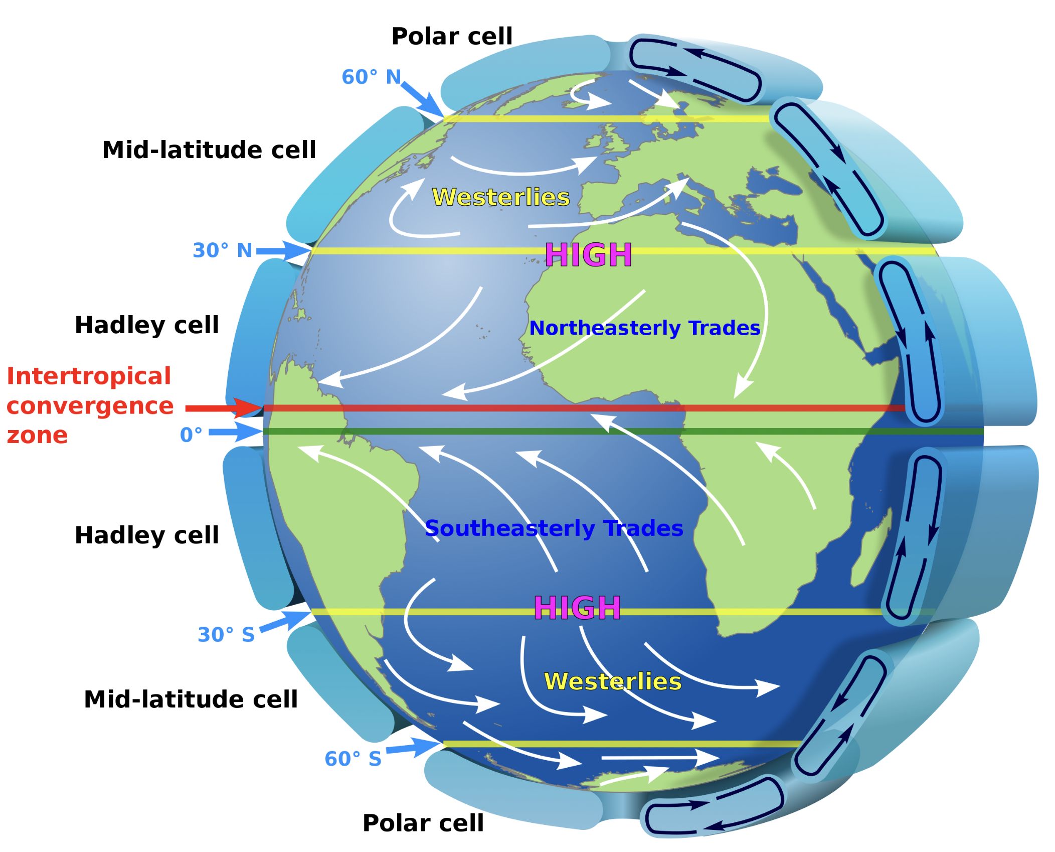
Fig. 6.15 Cartoon of the mean circulation in the atmosphere.#
In addition to thermal wind moving from west to east, the atmosphere also has a mean circulation in the \(z-y\) plane. We call this the meridional circulation. An important component of this is called the Hadley circulation after an English lawyer and amateur meterologist called George Hadley. This circulation is sketched in Fig. 6.15.
The following is a simple explanation for the mean Hadley circulation: As air near the equator is warmed by solar insolation, it rises until it reaches the top of the troposphere. Here the air is no longer buoyant enough to continue to rise and hence the air moves poleward in the upper troposphere. As the air flows north, it gradually sinks and then returns to the equator near the ground. The air moving equatorward at low levels is affected by the Earth’s rotation, causing it to veer to the west. The resulting winds blowing from east to west near the ground a low latitudes are the so-called `trade winds’.