4.3. River flows

Flow in a river

The previous lecture focussed on flow in the catchment towards a river. Some very simplified models for the surface run-off in terms of the rainfall flux were developed to help inform relationships between the rainfall rate and the rate at which this flows into a river.

To interpret these models of the surface runoff, we need a model for the flow in a river to understand if the river can accommodate the flow, or if it will overtop its banks and flood. As a simple model, a river has a cross-section area \(A(h)\) as a function of the water depth, and the water in the river moves downstream with speed \(u\). If the river inclination is \(\theta\) then the gravity force down slope is

\[F_g = g \sin{(\theta)} \rho A\]

and the drag force resisting this flow is

\[F_d = C_D \rho u^2 P\]

where \(P(h)\) is the wetted perimeter of the river bed and \(C_D\) is the drag coefficient of the river bed.

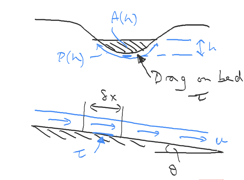
Fig. 4.13 The geometry of an idealised river bed. (NB \(\tau = C_D\))

If we balance these forces we find that the speed

\[u(h) = \sqrt{\frac{A(h)}{P(h)} \frac{g\sin(\theta)}{C_D}}\]

Derivation

Drag force

The inertia represents the force required to speed up or slow down the flow (i.e. the change in momentum); as fluid moves around an obstacle, it may change direction for example, over some length scale \(h\) comparable to the depth of the flow, and this requires a time \(\Delta t \sim \frac{h}{u}\), so the effective change in momentum with time (i.e. the force required) is

Units!

\[\begin{split} y &= \mathrm{s} \\ h &= \mathrm{m} \\ u &= \mathrm{m~s^{-1}} \\ \rho &= \mathrm{kg~m^{-3}} \\ C_D &= \mathrm{unitless} \\ g &= \mathrm{m~s^{-2}} \\ \theta &= \mathrm{radians} \\ q &= \mathrm{m^{2}~s^{-1}} \\ \end{split}\]

(4.7)\[\dv{\rho u}{t} \sim C_D \frac{\rho u}{\Delta t} \sim C_D \frac{\rho u^2}{h}\]

where \(C_D\) is a constant of proportionality; the drag coefficient, \(h\) the depth of the flow and \(u\) is the flow speed. There are published tables (e.g. Moody) for the drag as a function of the roughness of the bed, but a representative value for \(C_D\) may be 0.01-0.004.

Gravity force

If the gravity force per unit volume down-slope is \(\rho g \sin(\theta)\) for a slope of angle \(\theta\) then we can balance the forces on a volume of fluid. For a distance along the river \(\delta x\), with a cross sectional area \(A(h)\), we have a volume of fluid \(A(h) \delta x\), and hence a gravity force acting:

(4.8)\[F_g = \rho g \sin(\theta) A(h) \delta x\]

and similarly we have a drag force acting (assuming we take the area of the river to go as \(A(h) \sim P(h) \vdot h)\)

(4.9)\[F_d = C_D \frac{\rho u^2}{h} P(h) \vdot h \delta x\]

and so balancing these forces we get

(4.10)\[\begin{split}\begin{align} F_d = & F_g \\ C_D \frac{\rho u^2}{h} P(h) \vdot h \delta x = & \rho g \sin(\theta) A(h) \delta x \\ C_D u^2 P(h) = & g \sin(\theta) A(h) \end{align}\end{split}\]

and rearranging for \(u\) we get

(4.11)\[u = \sqrt{\frac{A(h)}{P(h)} \frac{g \sin(\theta)}{C_D} }\]

Reynolds Number

We can also use our intuition for the magnitude of the inertial force to derive the Reynolds Number, which identifies what kind of flow regime we are in. In contrast to our deep river, for a very thin film the viscous force from the ground will dominate the flow, and this has the form

Units!

\[ \mu = \mathrm{kg~m^{-1}~s^{-1}} \]

(4.12)\[F_v \approx \mu \frac{u}{h^2}\]

where \(\mu\) is the dynamic viscosity of the fluid, and again \(h\) is the depth of the flow.

Taking the ratio of the inertial ((4.7)) and viscous forces, we find

Units!

\[\begin{split} \Re &= \mathrm{unitless} \\ \end{split}\]

(4.13)\[\mathrm{Re} = \frac{\rho u h}{\mu}\]

which this is known as the Reynolds number.

If \(\mathrm{Re}\) is large (\(\mathrm{Re} \gt 1\)) it implies that the flow is dominated by the inertia. This corresponds to deep or fast flow. The Reynolds number can be \(10^5\) in a typical river. Shallower slow flow is more likely to have low Reynolds number (\(\mathrm{Re} \lt 1\)) and be controlled by the viscous drag. To estimate the transition point we can find the flux for which the depth of the current is comparable in the inertia dominated and viscous dominated flow (see the Examples Sheet).

And therefore the volume flow in the river is given as

\[Q = A(h) u(h)\]

In a specific example, we might consider that the river area \(A(h) = \alpha h^2\) and that the perimeter \(P(h) = \beta h\) (i.e. a triangular river) so that

\[Q(h) = \sqrt{\frac{\alpha^3}{\beta}} \sqrt{\frac{g\sin(\theta)}{C_D}} h^{\frac{5}{2}}\]

is the law for the flux in the river.

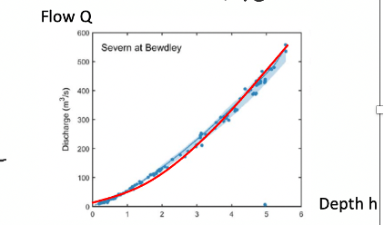
Fig. 4.14 The discharge rate \(Q\) in a river as a function of the water depth.

This provides a reasonable simplified model for the flow in many rivers, for example the chart in Fig. 4.14 compares this formula with data from the River Severn showing flow as a function of the water depth.

Critical flow rate for flooding

An initial result emerging from this model is that if the level of the banks are at \(z = h^*\) above the base of the river, where \(h^*\) is the height at which the water will overtop the bank, then the critical flow rate of water in the river above which it begins to flood is

\[Q^* = Q(h^*)\]

and we can link this back to our drainage basin model to predict when a river might flood based on rainfall.

If we want to use this model for the river flow to reduce the flood we see that the key controls we have are (a) raising the height of the banks; (b) deepening the river; (c) widening the river.

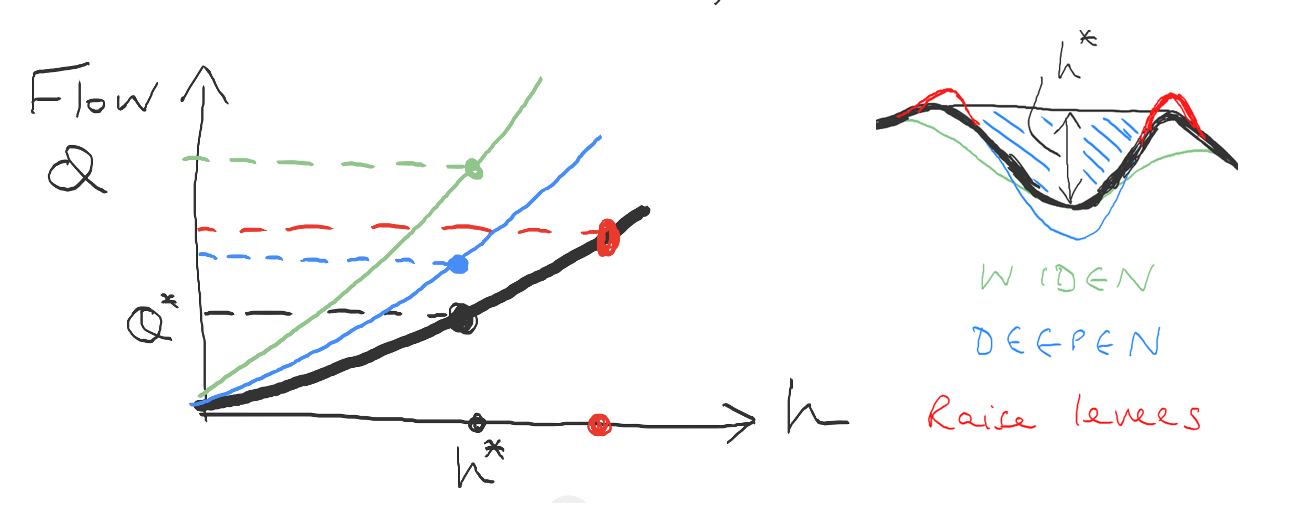
Fig. 4.15 An illustration of mitigation strategies to prevent flooding of a river.

Our earlier idealised models for the surface runoff identify how more intense and longer duration rain events lead to a greater flux reaching the river, and hence we can explore the type of rainstorm which will lead to the flux exceeding the maximum river flux in terms of the model for the runoff. Given statistics for the distribution of expected rainfall intensity and rainfall duration, it is then possible to design mitigation measures to reduce the flux arriving at the river from the run-off for a given rainstorm. There is then a cost benefit analysis to be carried out to determine the benefit of mitigating the flood risk for different intensity storms: this involves estimating the costs of the mitigation measures compared to the costs of the damage produced by the flooding multiplied by the risk of the flooding.

Coupled Model

If we combine the runoff model with the river model we find the following comparison plot, illustrating how different types of rainfall lead to different flow regimes (i.e. flooding or not)

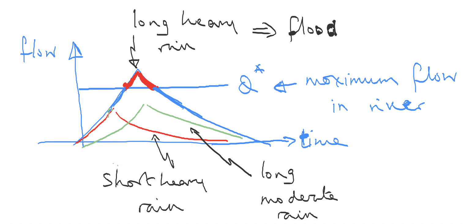
Fig. 4.16 A coupled river flow and flooding model

This model, although simplified, has features in common with the classical river hydrograph (Fig. 4.17), in which we plot the rainfall flux and the river flow rate as a function of time.

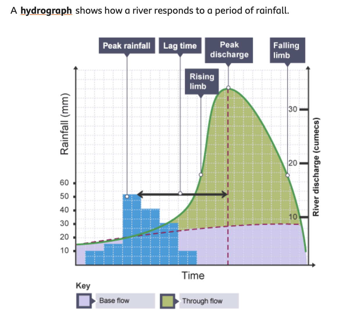
Fig. 4.17 A hydrograph showing the rainfall flux and the river flow rate as a function of time.