6.7. Stommel box model for ocean heat transport#
Recall from Fig. 6.5 that the ocean makes a non-trivial contribution to the global heat transport, particularly in the subtropics. Unlike the atmosphere, most of the oceanic heat transport is associated with the mean circulation, rather than eddies. In particular, currents that develop on the western sides of ocean basins make a major contribution to the heat flux. These western boundary current include the Gulf Stream in the North Atlantic and the Kuroshio in the North Pacific.
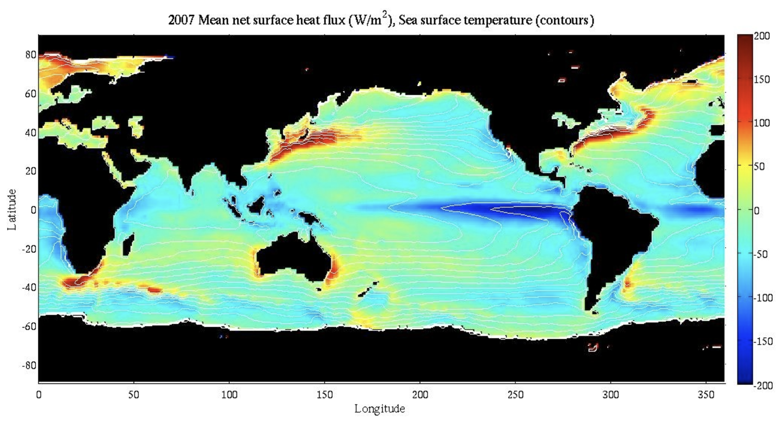
Fig. 6.22 Mean air-sea heat flux. Data from Yu and Weller, 2007. Positive values indicate heat transfer from the atmosphere to the ocean.#
As warm water flows polewards, it encounters cold air and heat is transferred from the ocean to the atmosphere. Fig. 6.22 shows the annual average net surface heat flux. The western boundary currents are highlighted as regions with large positive heat fluxes, indicating a large amount of heat going from the ocean to the atmosphere. Instantaneous heat fluxes can be much larger. For example, field work conducted in the Gulf Stream during the winter found ocean surface temperatures of 19-20\(^\circ\)C and air temperatures of \(1-2^\circ\)C with snow, sleet, and rain! The estimated net heat flux from the ocean to the atmosphere during this period was about 1000 W/m\(^2\).
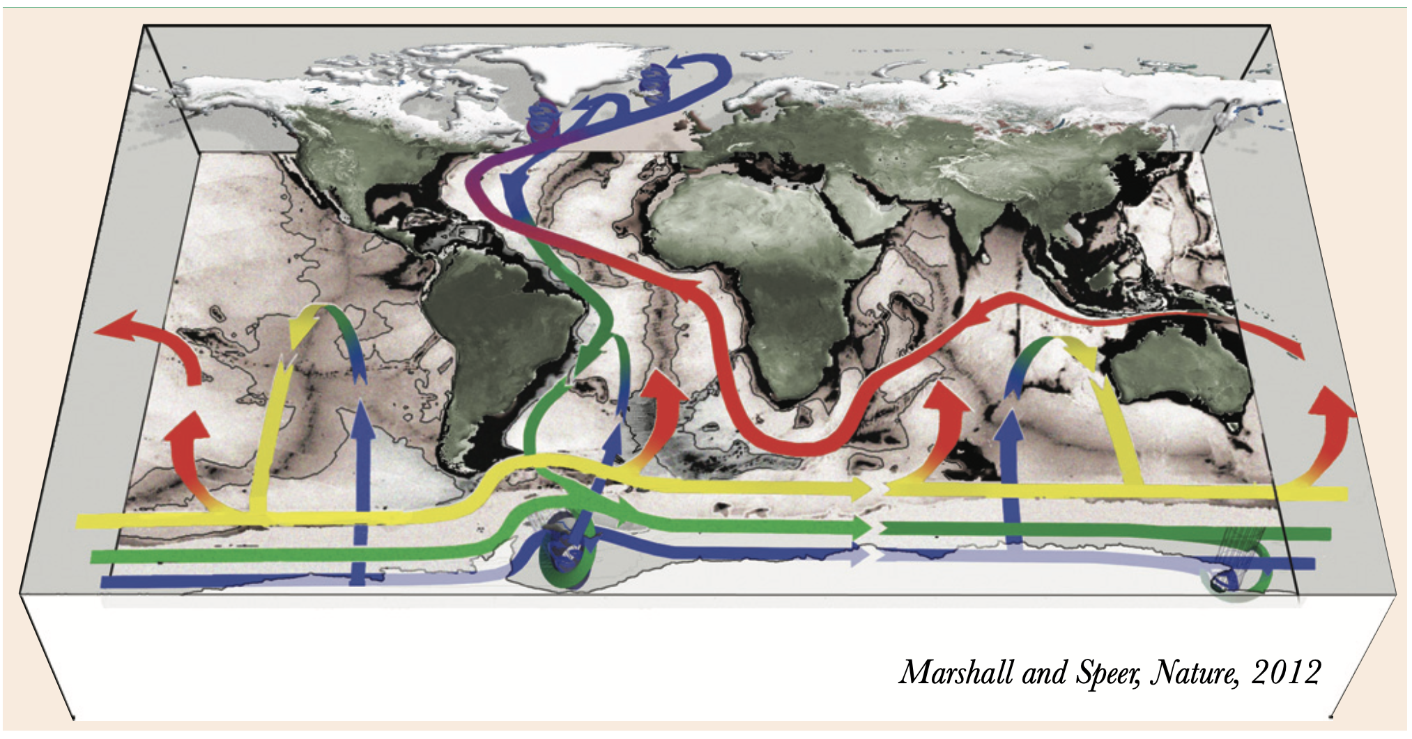
Fig. 6.23 Cartoon of the global meridional overturning circulation.#
When the near-surface water cools, it becomes more dense. Eventually the water becomes dense enough to sink into the interior of the ocean, where it returns to lower latitudes and gradually upwells. This circulation is called the Thermohaline Circulation, or THC, because both temperature (thermo) and salt (haline) control the density of seawater[1].
In this section, we will develop a box model for the Thermohaline Circulation and use it to investigate some important features of the large-scale ocean circulation and heat transport. In one of the practical sessions, we will construct a computer code to solve the box model equations numerically and we will use this to study the time evolution of the system in more detail. In the next two sections we will describe the physical mechanisms underlying the box model to help put it the model in context and to understand the parameter dependence of each of the terms.
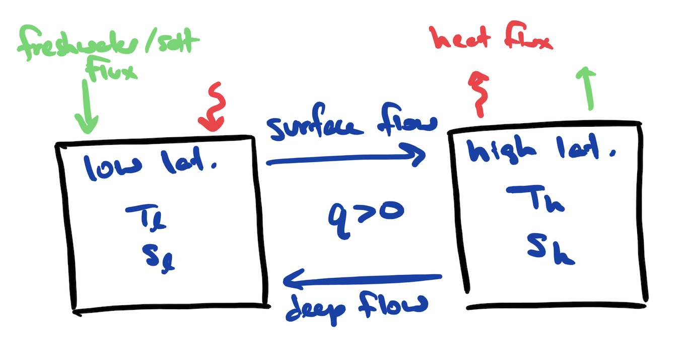
Fig. 6.24 Sketch of the Stommel box model for ocean heat transport.#
The model that we will use is sketched in Fig. 6.24. This is often called the `Stommel model’ since it was first proposed by Henry Stommel, a pioneering physical oceanographer at the Woods Hole Oceanographic Institute in Massachusetts, USA. Like the atmosphere box model that we saw in the last section, the Stommel model has two boxes - one for low latitudes (denoted with “l”) and one for high latitudes (denoted wth “h”). Each box represents the mean ocean properties (averaged in longitude and depth) in that region. As before, the high latitude box accounts for the ocean at high latitudes in the northern and southern hemispheres.
In the ocean, the density of seawater depends on the water temperature, salt content (or salinity), and pressure. The density is a nonlinear function of temperature and salinity, and the equation relating density to temperature, salinity, and pressure is called the equation of state. Since we are considering the depth-averaged water properties, we won’t explicitly consider the pressure dependence. To make the model simpler, we will use a linear approximation to the equation of state in the following form:
where \(\rho\) is the density, \(T\) is the temperature, and \(S\) is the salinity, and \(\rho_0\), \(T_0\), and \(S_0\) are constant reference values for the density, temperature, and salinity, respectively[2]. The coefficients in this equation are called the thermal expansion coefficient (\(\alpha\)) and haline contraction coefficient (\(\beta\)).
The arrows at the top of each box indicate fluxes between the ocean and atmosphere. The salt content in the ocean changes due to evaporation and precipitation. Although the rate of evaporation depends on the temperature of the atmosphere and the ocean (and the wind speed), we will assume that the net freshwater flux is constant and we will denote this by \(E\) (for evaporation). As an extension to the practical project, you could explore the effect of variable evaporation on the model results.
We will assume that the rate of heat transfer between the ocean and atmosphere is proportional to the difference between the ocean and atmosphere temperature in the high latitude or low latitude box. We will denote the temperate in the atmosphere above the low and high latitude boxes by \(\overline{T_l}\) and \(\overline{T_h}\). To model the heat exchange between the ocean and atmosphere, we use a ‘relaxation’ term which causes the temperature in the ocean to gradually ‘relax’ towards the temperature in the atmosphere. Specifically, in a model without any exchange between the boxes (\(q=0\)), the temperature in each box would evolve according to
where the subscript \(l,h\) indicates that the equation applies for \(T_l\) and \(T_h\). Solutions to this equation are of the form (see example sheet problem)
where \(C\) is the temperature at \(t=0\) (the initial condition). Note that to solve this equation we have assumed that the atmospheric temperature, \(\overline{T}_{l,h}\) is constant. From the form of Eq. (6.29), we see that the temperature in each box decays (or relaxes) exponentially from the initial temperature towards the atmospheric temperature at a rate set by \(\gamma\).
The last term that we need to specify is the transfer of water between the two boxes. This flux is intended to represent the Thermohaline Circulation (THC), which as we have said carries warm water from low to high latitudes near the surface, while returning at depth. The term \(q\) will denote the strength of this circulation, and when \(q>0\), the water will move as indicated in Fig. 6.24. Since the THC involves the water becoming more dense and sinking at high latitudes, we anticipate that the strength of the circulation will be proportional to the density difference between the high and low latitude boxes, i.e.
where \(k\) is a constant of proportionality, and we have used the linear equation of state to relate the difference in density to differences in temperature and salinity with \(\Delta T=T_l-T_h\) and \(\Delta S=S_l-S_h\) denoting the temperature and salinity differences between the low and high latitude boxes. Note from the form of Eq. (6.30) that \(q=0\) when \(\rho_l=\rho_h\). The circulation is non-zero when there are differences in temperature and/or salinity between low and high latitudes. Which of these factors is more important will depend on the climate state, and we will have the opportunity to explore this in the practical.
The heat flux carried out of a box is proportional to the product of the circulation strength (\(q\)) and the temperature of the outgoing box. Similarly, the salt flux is proportional to the product of \(q\) and the salinity of the outgoing box. This formulation requires knowledge of the direction of the flow, and hence our model will only be valid for \(q>0\) (the expected direction of the THC).
Putting this together, the equations for the Stommel model can be written:
where \(\Delta T=T_l-T_h\), \(\Delta S=S_l-S_h\), and \(q=k(\alpha \Delta T - \beta \Delta S)\) as defined above.
In the practical project, we will solve the equations for the Stommel model numerically. Here, we will look for steady state solutions in the limit when the ocean rapidly relaxes towards the atmospheric temperature. Specifically, let’s consider the limit when \(\gamma^{-1}\ll q^{-1}\) (or equivalanetly \(\gamma\gg q\)). In this limit, the ocean temperature will remain close to the atmospheric temperature, or \(T_l\simeq \overline{T}_l\) and \(T_h \simeq \overline{T}_h\). If we further assume that \(\overline{T}_l\), \(\overline{T}_h\), and \(E\) are all constant, then we can subtract the last two equations in the Stommel model to give
Taking the time derivative of Eq. (6.30) with \(d\Delta T/dt=0\) gives
Combining these two equations, we find that
We can write this as a single equation for \(q\) by re-arranging Eq. (6.30):
where \(\overline{\Delta T}=\overline{T}_l-\overline{T}_h\), \(\Delta T = \overline{\Delta T}\) from the assumption of \(\gamma^{-1}\ll q^{-1}\). Using Eq. (6.33) in Eq. (6.32) gives
Steady state solutions satisfy a quadratic equation where the right hand side of Eq. (6.34) is zero. Solutions to this quadratic equation are
An interesting feature of the Stommel model is that it has multiple equilibria. In fact, another pair of equilibria emerge if we allow \(q<0\). It turns out that two of these equilibria are stable, meaning that if the system is given a small perturbation to the equilibrium value (say \(q=q_e+\epsilon\) where \(\epsilon\) is small), then the solution will return to the equilibrium value \(q=q_e\). This is a very important result for our understanding of the climate system. It implies that the climate system can `switch’ between multiple states. This feature has been used to explain rapid climate variability during the Pleistocene. This has also led to concern that climate change could push the climate system to new state where the Thermohaline Circulation shuts down and the Earth is sent into a new ice age.