3.5. Floating ice shelves and the flow of glacial ice

In large ice sheets the flow of ice ultimately transports significant ice mass to the ocean, where the ice begins to float as an ice shelf. These ice shelves play an important dynamical role, particularly in western Antarctica, where they moderate the flow of ice from the continent to the ocean. In this lecture, we will describe the key dynamical balances governing the flow of ice shelves, along with their impact on grounded ice and the response of ice sheets to climate change (in particular the West Antarctic ice sheet).

A characteristic schematic of a marine ice sheet is shown in Fig. 3.23. Here a grounded ice sheet flows into the ocean. At the grounding line the ice begins to float and from there the ice floats and flows onto the ocean as an ice shelf.

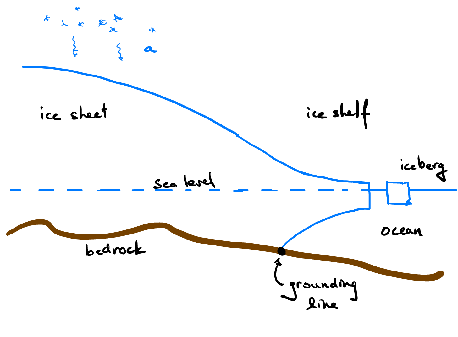
Fig. 3.23 Schematic of a marine ice sheet, including flow from the grounded ice sheet across the grounding line to the floating ice shelf.

The flow in the ice shelf is again long and thin, and hence the pressure is to leading order hydrostatic within the ice shelf. Hence, flow within the ice shelf is predominantly driven by hydrostatic pressure gradients. However, since the ice is now floating on the ocean there is negligible stress exerted by the ocean below, and by the atmosphere above. Hence, the velocity within the ice shelf is uniform in the vertical, varying only in the lateral dimensions (\(x\) and \(y\) in the coordinates used here).

The flotation condition

Ice floats on the ocean as it is less dense than ocean water. In general, ice has a density of approximately \(\rho = 917\ \mbox{kg m}^{-3}\) while, for typical ocean salinities, sea water has a density of \(\rho_w = 1020 - 1030\ \mbox{kg m}^{-3}\) (we’ll typically use a value of \(\rho_w = 1025\ \mbox{kg m}^{-3}\)).

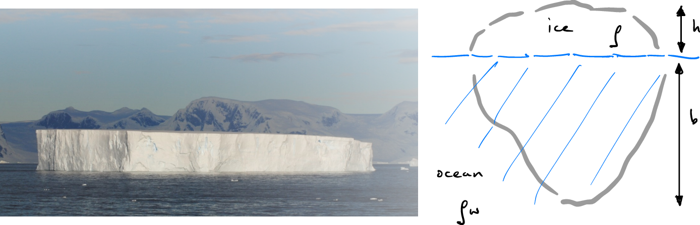
Fig. 3.24 The flotation of an iceberg in ocean water.

The depth to which ice floats in ocean water is given by Archimedes principle, which states that {\it a floating body displaces its own weight in water.} An equivalent approach to understanding this principle is to note that the ocean and the ice may be stationary when floating, so the pressure in both the ice and the water are hydrostatic. Hence, for an iceberg floating a distance \(h\) above the water, with a depth \(b\) submerged the equilibrium between ocean and ice may be written as

\[\rho_w g b = \rho g (h+b),\]

and hence

\[h = \frac{\rho_w-\rho}{\rho}b \simeq \frac{1}{9} b.\]

When applied to the transition from grounded ice sheet to floating ice shelf, this implies that the ice grounding line position is determined by the first point at which the base of the ice is equal to the depth of the ocean water,

\[b(x_G) = \frac{\rho}{\rho_w-\rho} h(x_G) = d(x_G),\]

where \(d(x_G)\) is the depth of the ocean, evaluated at the grounding line \(x_G\).

Grounding line stability

From the previous lecture on grounded ice sheets, we know that the flux of ice on land is driven by hydrostatic pressure gradients, and limited by the (vertical) viscous shear in the ice. This leads to a parabolic velocity profile in the ice, which implies that the flux of ice within the ice sheet is given by

\[q = -\frac{\rho g}{3\eta}(h+b)^3\frac{\partial h}{\partial x}.\]

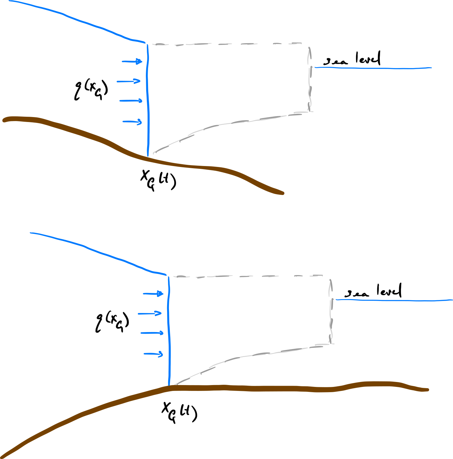
Fig. 3.25 Groundings lines on prograde (top) and retrograde (bottom) slopes, illustrating the stability of the grounding line.

The stability of grounding lines on either prograde (sloping down into the sea) or retrograde (sloping down into the ice) beds may be argued as follows. In both cases the argument relies on the flux across the grounding line increasing with increasing ice thickness.

For prograde slopes, an increase in the grounding line position corresponds to deeper water depths and hence a larger ice thickness (in order to satisfy the flotation condition). These larger thicknesses result in a greater flux across the grounding line, and this increased mass loss thins the ice sheet behind the grounding line. As a result the ice thickness thins at the grounding line and, again because of the flotation condition, the grounding line retreats. The prograde slope therefore has a negative feedback on grounding line migration.

In contrast, for retrograde slopes an increase in the grounding line position leads to shallower water depths and hence a thinner ice thickness, as determined by the flotation condition. This thinner ice thickness means that the flux across the grounding line is reduced, and hence mass can more rapidly build in the ice sheet. As a result of the excess mass in the ice sheet this drives the grounding line to advance, leading to yet shallower water depths, et cetera. The retrograde slope therefore has a positive feedback on grounding line migration.

The stability of the grounding line position suggests there are two physical processes setting the grounding line position. First, the grounding line position is determined by the flotation condition (Archimedean buoyancy). Second, it is a force balance at the grounding line that plays the second role in dynamically determining the flux of ice across the grounding line, and hence its position. Hence, given the topography of the bedrock the grounding line is where both flotation and force balance are satisfied and hence where both the depth and flux are prescribed.

Back stresses on the ice sheet

The back stress on the ice sheet is the force applied by the ice shelf on the ice sheet at the grounding line. For an ice shelf which simply extends into the ocean, and hence makes no contact with other points in the bedrock, the shelf is unable to exert a force on the ice at the grounding line (it is freely floating). Instead, it simply transmits the hydrostatic pressure from the ocean to the grounding line.

In contrast, if the shelf makes contact with pinning points - be they submerged islands, high points in the ocean bathymetry, or side walls of a fjord - then force exerted by the ground on the shelf may be transmitted back to the grounding line. This force back to the grounding line is termed a back stress, and it effectively thickens the flow at the grounding line (you can think of it as the additional stress exerted by the pinning points cause the viscous flow to back up behind the pinning point). Thickening of the ice at the grounding line causes the grounding line to advance, on either prograde or retrograde slopes, and so ice shelf buttressing acts to significantly stabilise ice shelves. If the warm (saline) ocean waters intrude under the ice shelves, there may be enhanced melting which can act to decrease the buttressing of the ice shelves, thus destabilising the grounding lines particularly in areas of retrograde bed slopes. This is what appears to be happening at Pine Island glacier (PIG) and Thwaites glacier on the western margin of Antarctica.

Buttressing of ice shelf flow

Let’s consider a specific case of ice shelf buttressing in a long fjord. A particular case in point might be Jakobshavn (or Ilulissat) glacier which is a significant outlet glacier on Greenland’s western margin. We’ll approximate the geometry of the fjord (narrow but deep bay) as a channel of width \(W\) through which a floating ice shelf (or ice tongue) flows.

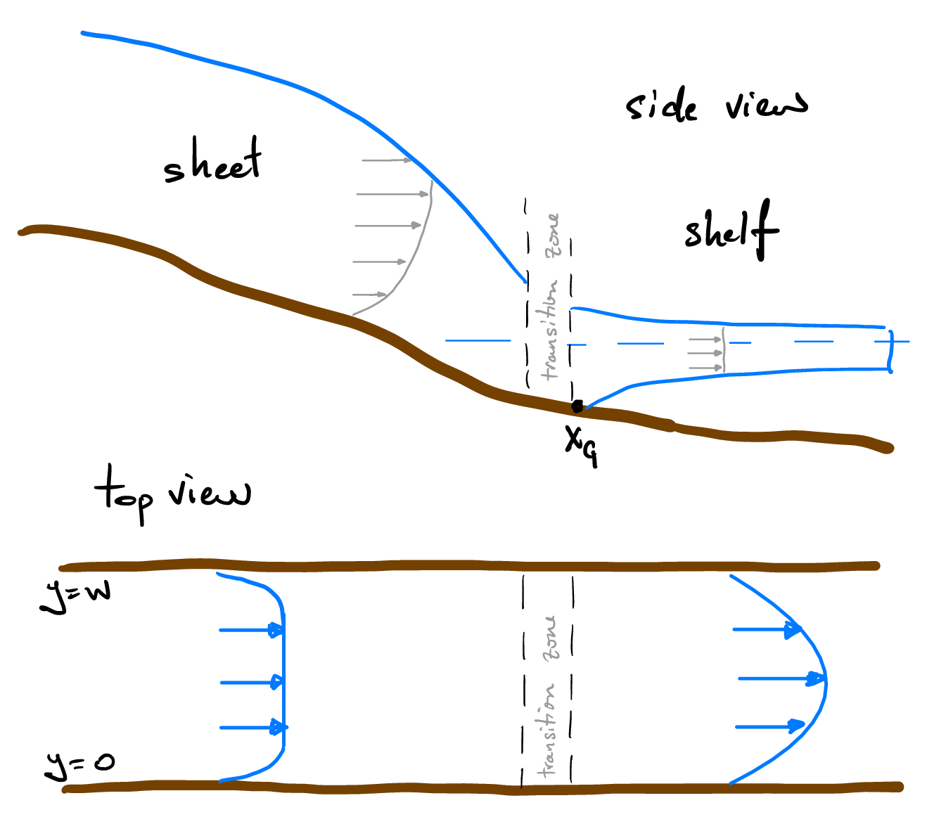
Fig. 3.26 The buttressing of an ice sheet flowing in a long channel of width \(W\).

Once the ice passes the grounding line and begins to float, there are no substantial stresses exerted on the ice shelf from the atmosphere or ocean, so the ice velocity \(u\) does not depend on depth and is instead a plug flow (uniform in depth) only depending on the lateral coordinates, \(x\) along the channel and \(y\) across it. To solve for the velocity profile we can use the same balance between pressure gradients and viscous shear we used for ice sheets,

\[\frac{\partial p}{\partial x} = \eta\frac{\partial ^2u}{\partial y^2},\]

now written as a balance between the pressure gradient down the channel (in the \(x\)-direction) balanced against viscous shear across the width of the channel (in the \(y\)-direction). We can integrate this expression twice, applying the boundary conditions that the velocity is zero on the channel walls,

\[u(y = 0) = u(y= W) = 0,\]

to find the expression for the ice velocity in the channel,

\[u = - \frac{1}{2\eta}\frac{\partial p}{\partial x}y(W-y).\]

We may note that the flow of the floating ice is mainly horizontal (no vertical velocity) and hence the pressure is nearly hydrostatic,

\[p = p_0 + \rho g (h-z),\]

where \(p_0\) is atmospheric pressure, \(\rho\) is the density of ice, \(g\) the gravitational acceleration, and \(h(x)\) the thickness which is predominantly a function of position within the channel. Hence, the ice velocity within the channel may be expressed as

\[u = -\frac{\rho g}{2 \eta}\frac{\partial h}{\partial x}y(W-y).\]

Finally, given the model for the ice velocity within the channel we may calculate two important quantities. First, we can calculate the flux through the shelf, which is the depth and width integral of the velocity,

\[q = \int_0^W (h+b)u\, dy = \frac{\rho g W^3}{12 \eta}(h+b)\frac{\partial h}{\partial x}.\]

Secondly, we can calculate the total force the buttressed shelf exerts on the ice sheet at the grounding line. This is equivalent to calculating the total viscous shear on the ice shelf (that viscous shear is what is holding back the ice). Hence the buttressing (acting in the negative \(x\) direction) is

\[- B = \frac{1}{W}\int_{x_G}^{x_N}(h+b)\frac{\partial p}{\partial x}\, dx = \frac{1}{W}\int_{x_G}^{x_N} (h+b)\eta \left[\frac{\partial u}{\partial y}\right]^{y = W}_{y = 0}\, dx.\]

This buttressing force acts to slow down the velocity of the ice, thickening the ice in the channel and hence at the grounding line. However, since the grounding line is constrained to be at the point of flotation (constrained by the densities of ice and water) buttressing tends to advance the grounding line, so can mitigate against the instability of the grounding line on retrograde slopes.

Two important examples mentioned in lectures of the buttressing of ice sheets by ice shelves are the breakup of the Larsen B ice shelf in 2002 which led to the speedup of the feeder glaciers along the Antarctic peninsula, and the response of the Rutford ice sheet to ocean tides.