6.3. Scales of motion in the atmosphere and ocean#
As we can see from the definition of the Rossby number, \(\mbox{Ro}\equiv U/(fL)\), small-scale motions in the atmosphere and ocean tend to be relatively unaffected by the Earth’s rotation since we might expect that \(\mbox{Ro}\gg 1\) when \(L\) is small. When \(\mbox{Ro}\simeq 1\), the two terms on the LHS of Eq. (6.6) will be comparable in magnitude. This happens when the characteristic lengthscale is \(L=U/f\). Motions with characteristic lengthscales larger than \(U/f\) will be strongly affected by the Earth’s rotation, while motions with on scales smaller than \(U/f\) will be relatively unaffected by the Earth’s rotation.
When \(\mbox{Ro}\ll 1\), Eq. (6.6) is approximated by
This state is called `geostrophic balance’. Since the time-derivative is neglected in this limit, this describes an equilibrium state where the velocity balances the pressure gradient through the Coriolis acceleration. Large-scale flows in the ocean and atmosphere tend to be close to geostrophic balance.
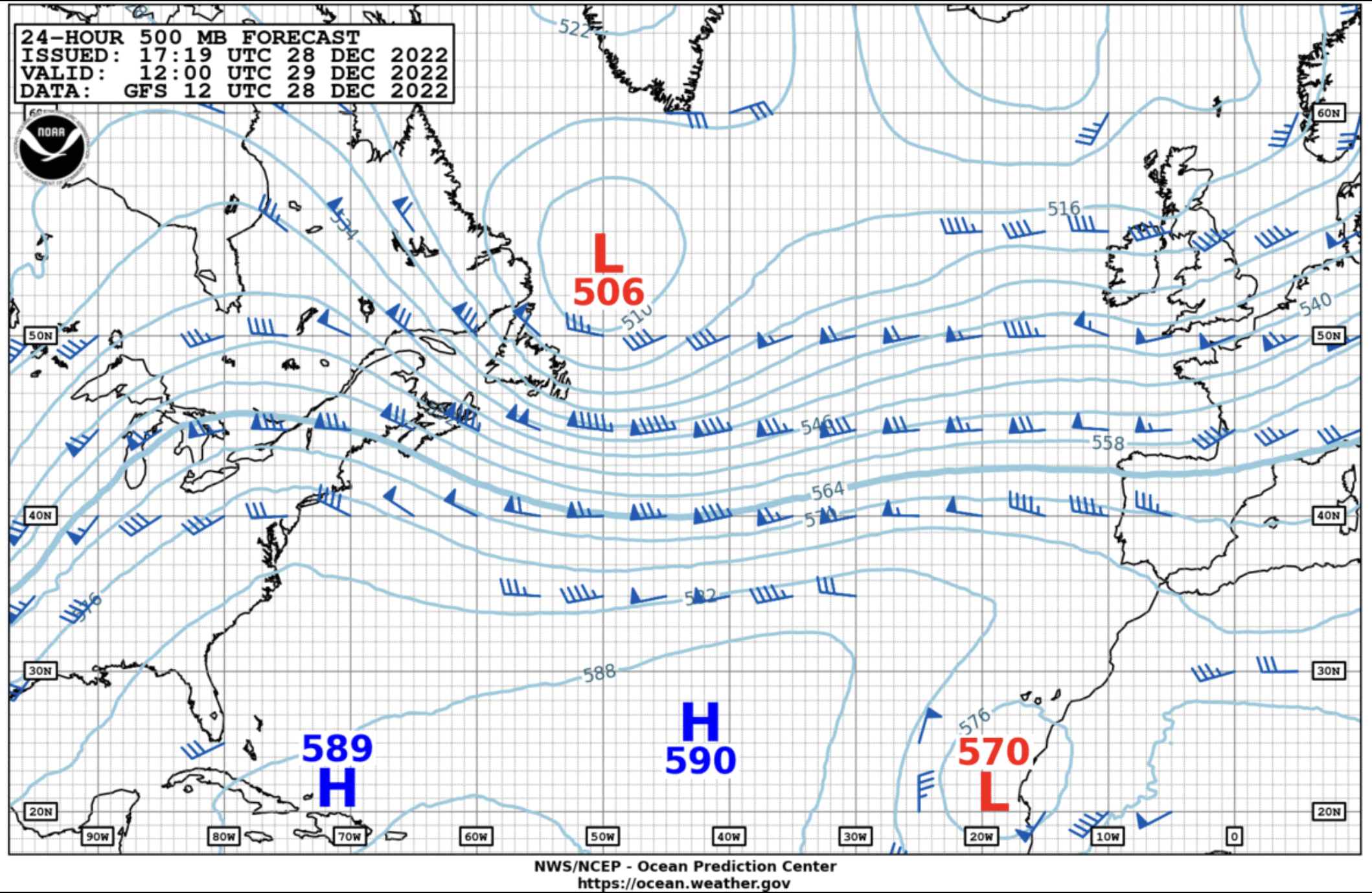
Fig. 6.10 Weather forecast chart for December 2022 showing pressure (contours) and wind (quivered arrows).#
Eq. (6.7) can be re-written
Therefore, the velocity in geostrophic balance is perpendicular to \(\nabla p\) and parallel to contours of constant pressure. Fig. 6.10 shows a weather forecast for the North Atlantic. The wind (quivered arrows) closely follows pressure contours, consistent with geostrophic balance. The magnitude of the velocity in geostrophic balance is proportional to the pressure gradient. In Fig. 6.10, stronger winds will occur where the pressure contours are closer together.
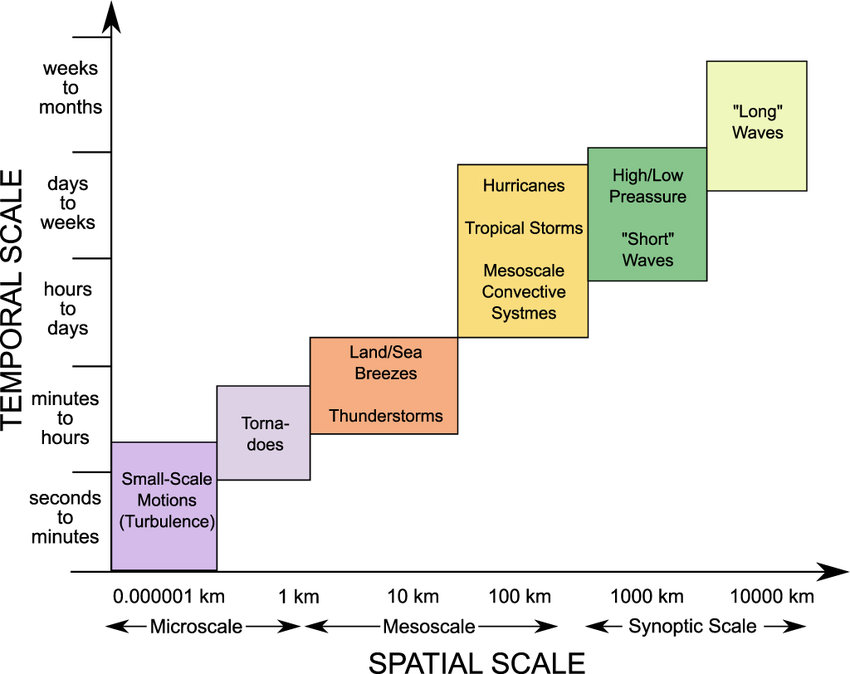
Fig. 6.11 Length and time scales of various atmospheric processes (not examinable). From Brisch and Kantz, 2019#
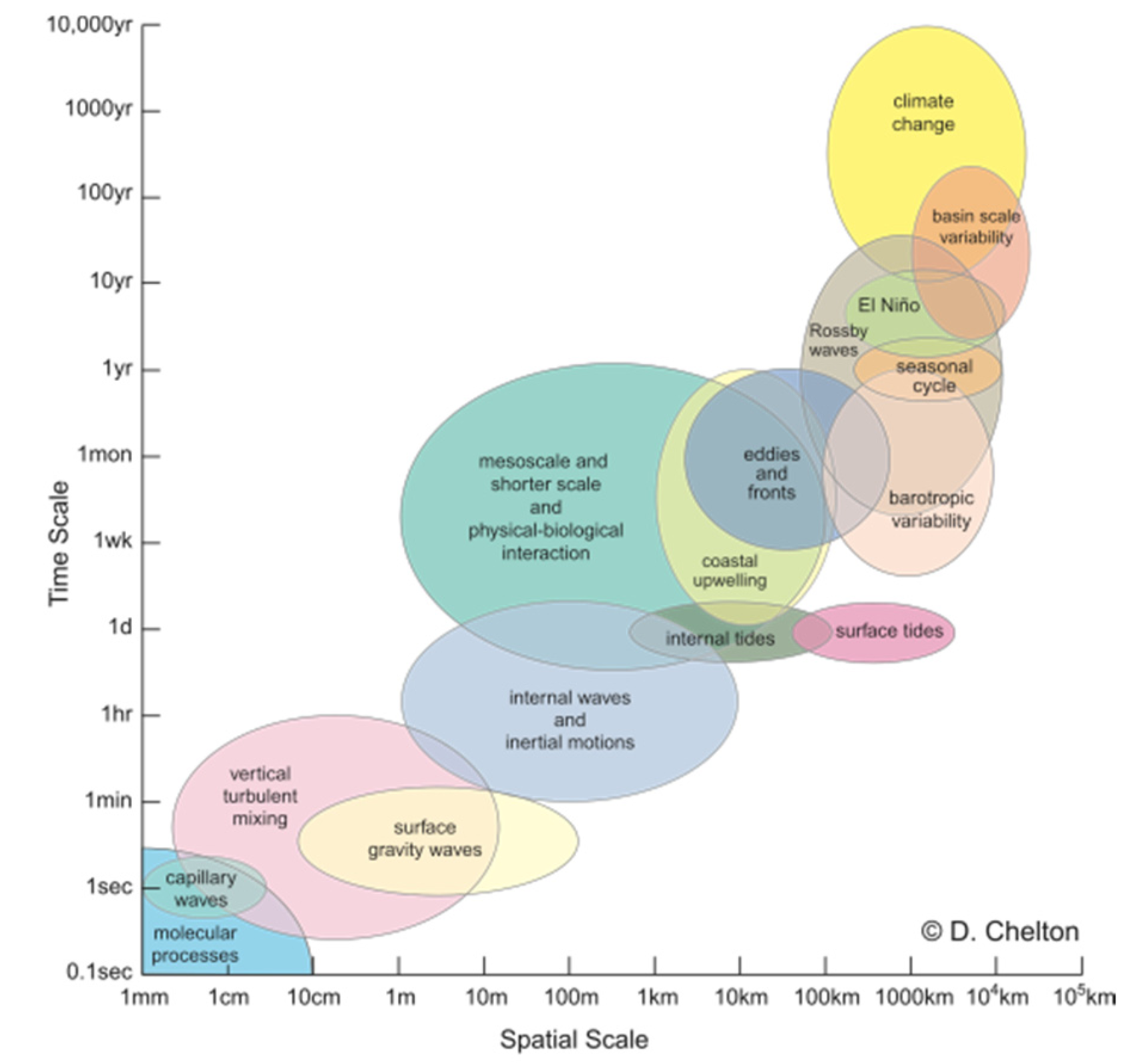
Fig. 6.12 Length and time scales of various ocean processes (not examinable). From Cronin et al., 2012 and D. Chelton.#
Fig. 6.11 and Fig. 6.12 show the length and times scales of various processes in the atmosphere and ocean (you will not be expected to remember these names or scales). A typical wind speed in the atmosphere is \(\sim 10 \mbox{m}/\mbox{s}\). The Coriolis parameter is \(f\simeq 10^{-4} \mbox{s}^{-1}\) at mid-latitudes. With these values, \(U/f\simeq 100 \mbox{km}\) in the atmosphere. Because this scale sits between large scale motions where the Earth’s rotation plays a large role and small scales where it is negligible, processes at this scale are call ‘meso’ (meaning middle) scale. Weather systems typically have a horizontal scale of \(\sim 1000 \mbox{km}\). With wind speeds on the order of 10 \(\mbox{m}/\mbox{s}\), weather systems typically have \(\mbox{Ro}\ll 1\) and hence are close to geostrophic balance (this is one reason why weather maps often show contours of pressure.) The advective timescale for weather systems at this scale is \(T=L/U\simeq 1\mbox{ day}\). This partly explains why weather patterns typically last for a few days.
Currents in the ocean are generally slower than wind in the atmosphere. A typical current speed in the ocean is \(U\sim 0.1 \mbox{m}/\mbox{s}\). Hence, \(U/f\sim 1 \mbox{km}\) in the ocean. The ocean contains eddies with typical sizes of \(\sim 100 \mbox{km}\). Since this corresponds to the atmospheric mesoscale, these ocean eddies are called ‘mesoscale eddies’ despite the fact that they are characterised by \(\mbox{Ro}\ll 1\). Like atmospheric weather systems, mesoscale eddies are typically close to geostrophic balance.
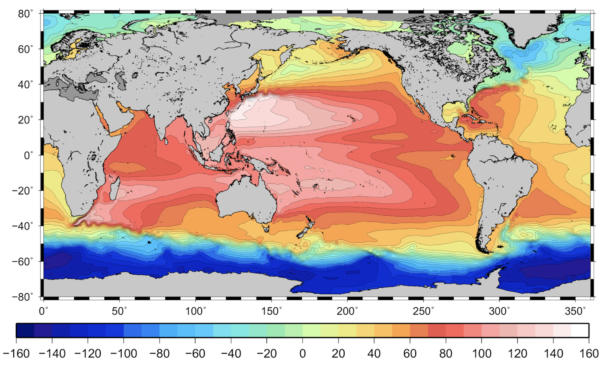
Fig. 6.13 Mean sea surface height (departure from the stationary geoid) in cm.#
Large-scale pressure gradients within the ocean are usually associated with changes in temperature (and hence density) and/or surface elevation. As an example, let’s look at how variations in the surface height of the ocean correspond to large-scale ocean currents. In a state of hydrostatic balance, the vertical pressure gradient force is balanced by the buoyant force acting on a fluid parcel, or
(Recall that we have seen this balance in the cryosphere and atmospheric chemistry lectures.) By convention, when studying the ocean we often let \(z=0\) correspond to the sea level for a stationary ocean (with a constant geopotential height). The positive \(z\) direction still points up so that \(z<0\) in most of the ocean. Let \(z=\eta(x,y,t)\) correspond to the height relative to the stationary geoid. For now, let’s assume that the density of seawater (\(\rho\)) is constant. Then, if we integrate Eq. (6.9) from a height \(z\) to the top of the ocean \(\eta\), we get
For simplicity, let’s also assume that \(p_{A}\) is constant. Using Eq. (6.10) in the relation for geostrophic balance (Eq. (6.7)) then gives
From this equation, we see that the surface height plays a similar role to the pressure for ocean currents that are in geostrophic balance, i.e. the velocity will follow contours of constant surface height and the speed is proportional to the gradient in surface height.
Fig. 6.13 shows the mean (time-averaged) surface height, \(\eta\). The Gulf Stream is visible as a large gradient in the sea surface height in the North Atlantic. The sea level to the south of the Gulf Stream can be about 1m higher than the sea level to the north of the Gulf Stream. The resulting pressure gradient within the ocean is associated with geostrophic current speeds in excess of 1 m/s. The large gradient in surface height in the Southern Ocean is associated with the Antarctic Circumpolar Current - a major current system which flows eastward, circling Antarctica. In between the other continents, the surface height contours form closed ‘loops’. This is the imprint of large ocean ‘gyres’. Notice also that the sea level is significantly higher on the western sides of the ocean basins at mid-latitudes. We will discuss these features in some depth in a few lectures.