8.3. The Methane Budget

To understand why there was a pause in the increase in methane concentrations in the atmosphere from 2000-2006, we need to better understand the balance of the sources and sinks of methane to the atmosphere from the land surface. This quantification is done largely through two means – one is top down inventories of the methane budget and the other is bottom up inventories of the methane budget. These have multiple overlapping temporal and spatial scales and involve a range of different types of measurements and models (Fig. 8.19), and when combined allow us to understand the balance between the sources and sinks of methane to the global budget.

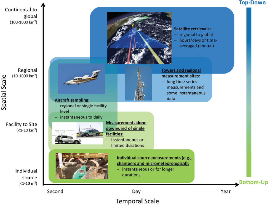
Fig. 8.19 The spatial and temporal scale of methods used to measure methane.

Top-Down Inventories

Top-down estimates of methane emissions combine atmospheric observations with inverse models, which are used to estimate where the emissions have derived. Methane absorbs well in the shortwave infrared (SWIR, Fig. 8.20). There are now many satellites that measure methane concentrations daily with near global coverage. Methane concentrations can also be measured by research aircraft although they don’t have nearly the same coverage as satellites.

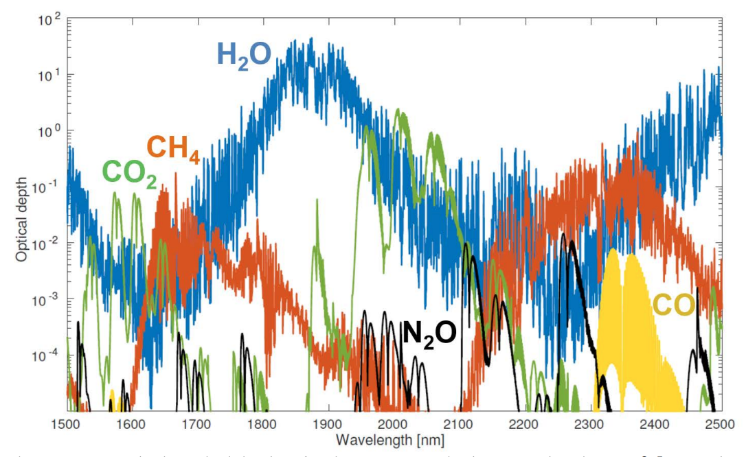
Fig. 8.20 Atmospheric optical depths of major trace gases in the spectral region 1.5-2.5 μm. The calculation is for the US Standard Atmosphere (Anderson et al, 1986) with surface concentrations adjusted to 399 ppm CO₂, 1.9 ppm methane, 330 ppb N₂O and 80 ppm CO. The line-by-line data are smoothed with a spectral resolution of 0.1nm (full width at half maximum). Figure from Jacob et al., 2016.

Knowing the methane concentration is half the battle, the other half is figuring out where it came from. This requires atmospheric chemistry models, and a particular class of model called inverse models (Fig. 8.21). Most of the models we have been looking at throughout QES are forward models, which step forward in time, iterating some parameter or variable.

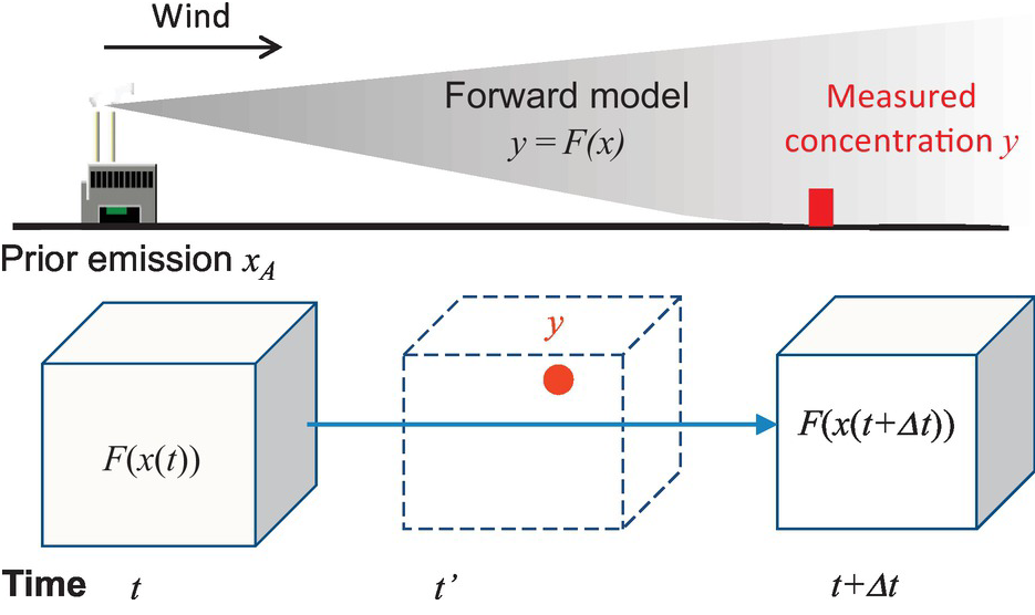
Fig. 8.21 Schematic of an forward model.

Inverse models start with the measurement and then run the model backwards to figure out where the source is (and then they can attribute it to what generated the source). The issue becomes that the lengthscale for the observations is often very different to the lengthscale for the source. For example, a pipe leak (the source) versus the resolution of a satellite (the observation) or reverse in the case of a wildfire (the source), versus a research flight (the observation).

These top down approaches have allowed for a global methane budget to be calculated (Fig. 8.22). Top down approaches do a pretty good job of balancing the sources and the sinks of methane to the atmosphere, with a small excess in the sources driving the increase observed in the atmosphere.

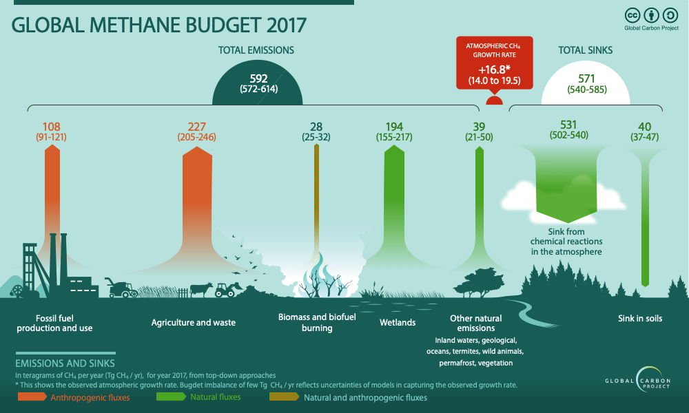
Fig. 8.22 The global methane budget in 2017, measured using top-down methods.

Bottom-Up Inventories

The other way to approach the methane budget is through the use of bottom up techniques. Bottom up techniques are based on emission inventories, biogeochemical models of methane emissions related to different environments, and direct measures of photochemical oxidation of methane in the atmosphere (Fig. 8.23). Bottom up techniques are data-heavy, but feed into the satellite measurements of methane emissions. Bottom up techniques involve multiplying the activity by the emission factor. The activity is essentially how much you have of something, and the emission factor is how much methane that something emits per unit time. For example, livestock emissions are from methane produced in the stomach of cows, and are measured at the point source by estimating the methane concentration that the cow breathes out multiplied by the number of cows (the ‘activity’). We can consider how bottom up source estimates are measured by considering each of these in turn.

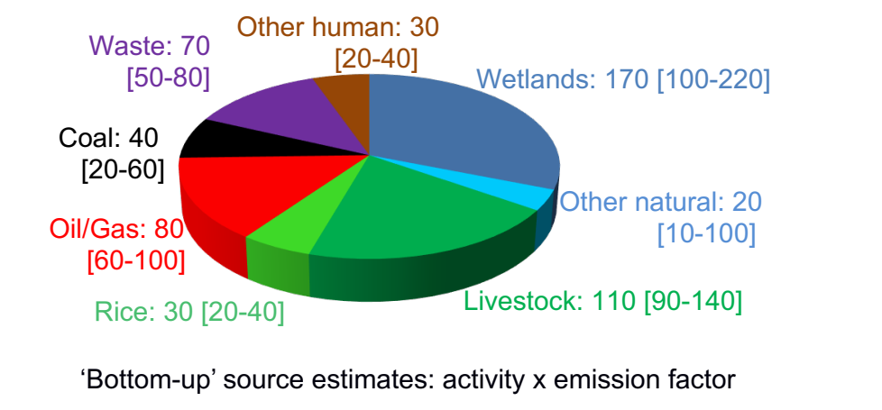
Fig. 8.23 A summary of ‘bottom-up’ estimates of methane sources.

The flux of methane from oil and gas production has been hard to quantify, and much recent work has suggested that pipelines and oil fields are far leakier than was previously thought. The main issue is that there are many places along the oil, gas, and coal production path where methane can be leaked to the atmosphere (Fig. 8.24).

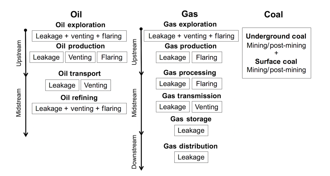
Fig. 8.24 Mechanisms of methane release from hydrocarbon extraction and processing from Scarpelli et al. (2020).

Landfills are another major source of methane, and recently the use of gas produced in landfills as an energy source has become more common and mainstream. However landfills continue to emit methane to the atmosphere in large quantities. Measuring this can be done with surface instrumentation, from the very small scale (someone walking around with a monitor) to the larger scale (using eddy covariance techniques, or optical plume monitoring), to aircraft measurements with inert tracer gases that are put in the land fill and then traced by aircraft monitoring (Fig. 8.25).

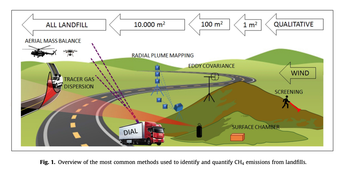
Fig. 8.25 The range of areas that can be covered by different monitoring techniques, from Monster et al. (2019).

Finally, for landfills, and more broadly soils including wetlands and rice paddies, a very common technique is to use a flux chamber, where the concentration of the gas coming off the soil is measured as it fills the chamber, allowing you to determine the amount of methane produced by an area over a known time period.

Measuring Fluxes

Recall that the overall flux of a compound of interest is the flux related to advection and the flux related to diffusion. The flux related to advection is calculated knowing the velocity of a fluid (air, water) and the concentration of the element/compound of interest in that fluid.

\[F_a = v C\]

Where \(F\) is the flux, \(v\) is the velocity of the fluid (m s^-1) and \(C\) is the concentration of that element or compound in the fluid (kg m^-3). This gives units of Flux of kg m^-2 s^-1 – or an amount (kg) per unit area (m^-2) per unit of time. The advective flux is what moves a plume of methane from point A to point B, or moves the concentration of a contaminant, say a toxic metal, down a river from point X to point Y.

In addition to advection, there is a flux related to diffusion, which we have seen earlier this term in Global Environment, and was encountered in Michaelmas term as well. At its essence, diffusion refers to the ‘random walks’, or the random movement of particles due to kinetic energy, and results in the net movement of the diffusing substance from a higher to a lower concentration.

Mathematically the diffusive flux is given by:

\[F_d = -D \dv{C}{x}\]

Where \(D\) is the diffusion coefficient, which is a property of the compound of interest (e.g. methane in soil) as well as of the media through which it is moving (the soil, and how porous it is, and what the shape and connectivity of those pores are). \(D\) has units of m2 s^-1, and \(\dv{C}{x}\) is the gradient of the gas concentration in the soil. By convention, the diffusive flux is negative because depth is positive going down into the soil.

The diffusion coefficient takes into account the soil tortuosity and porosity, and is often calculated as

\[D = D_0^{\tau^2(f(e))}\]

where \(D_0\) is the diffusion of gas in air (m² s^-1), \(e\) is the soil air-filled porosity (m³ air/m³ soil), and \(\tau\) is the tortuosity of the soil. Tortuosity gives us a sense of how straight a path is through the soil matrix. It is the ratio of the actual flow path length to a straight path length and formulations for the tortuosity include the porosity (\(e\)). This is illustrated in Fig. 8.26.

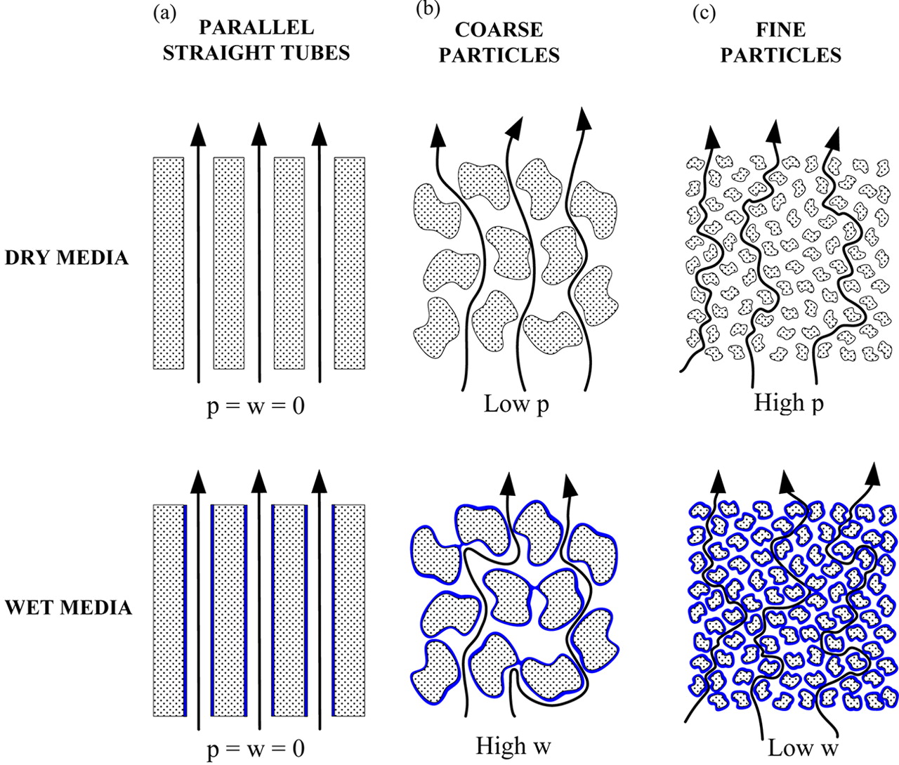
Fig. 8.26 Variations in tortuosity \((\chi)\) of a soil matrix.

In the case of the chamber measurements, we often assume that the advective flux in the soil is zero, and we measure the diffusion of gas into the chamber. This is generally a reasonable assumption, as there is very little air movement within soil! In this case, diffusive fluxes should account for the total emission from the soil, and should be equal to the net production of the gas in the soil (where net production is total production minus total consumption). What we measure in the chamber is the rate of increase in gas concentration with time (\(\dv{C}{t}\)) and then multiply this by the volume/area, to give the flux (Fig. 8.27)

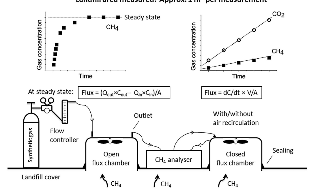
Fig. 8.27 Measuring methane with flux chambers. Units: \(\dv{C}{t}\) = concentration (kg m^-3) per time, Volume/area is m³ m^-2, overall the flux is kg m^-2 time^-1.

The other way to calculate the flux out of soils is to measure the concentration gradient itself, and estimate the porosity (and tortuosity) to calculate the flux from within the soil.

When we put all of this together we get overall estimates and maps of sources of methane to the atmosphere, and these can be attributed to various regions of the world where that methane is coming from (Fig. 8.30).

We can also use measurements and models to try to understand the amount of OH^- radical in the atmosphere, which is the dominant sink for methane (~90%). Reaction rates of methane oxidation are strongly linked to local changes in OH^- concentration. Two approaches derive estimates of OH^- quantity in the atmosphere:

1. Chemistry climate models that includes hundreds chemical reactions between numerous species

2. Methyl-chloroform (MCF) observations. Methyl chloroform is an anthropogenic pollutant that reacts with OH with a lifetime of 5 years. There have been no sources of MCF since it was banned in 1996.

Both approaches derive a 10-15% uncertainty on global OH^- mean concentrations.

Having gone through the various methods that are used to quantify methane emissions, we can compare the overall budget for methane sources and sinks calculated through bottom up (Fig. 8.28) approaches versus those calculated through top down (Fig. 8.22) approaches. This comparison shows us that bottom up approaches suggest a far larger source of methane to the atmosphere, greatly out of balance with the sinks of methane from the atmosphere.

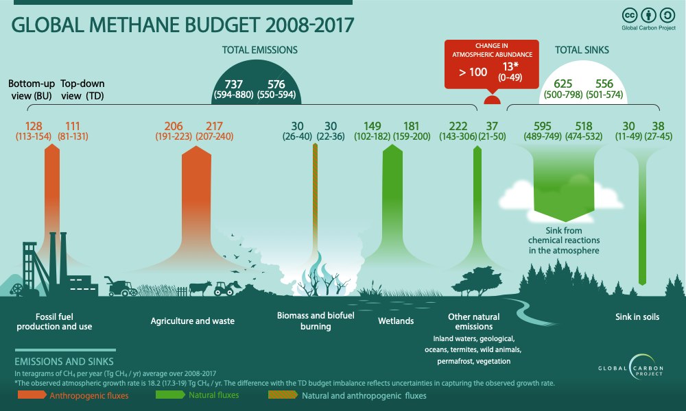
Fig. 8.28 A comparison of the global methane budget estimated from bottom-up and top-down measurements.

In summary:

• Global emissions:

  • 576 TgCH4/yr [550-594] for Top Down

  • 737 TgCH4/yr [594-881] for Bottom Up

• Top down and bottom up estimates generally agree for agricultural emissions

• Estimated fossil fuel emissions are lower for top down than for bottom up

• Estimated wetland emissions are higher for top down than for bottom up

• Large discrepancy between top down and bottom estimates for freshwaters and natural geological sources (“other natural sources”)

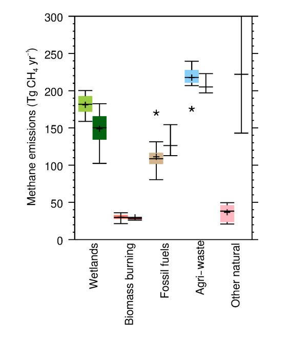
Fig. 8.29 A summary of methane emissions from different environments,

Finally, We can return to the question of what caused the pause in the increase in methane emissions between 2000-2006 by looking in detail at these emissions inventories and parsing them out globally.

When we compare 2000-2006 to 2017 (Fig. 8.30), we see that there has been a massive increase in emissions from agriculture and waste as well as fossil fuels. More recent work suggests that most of the increase is due to agriculture and waste. Worryingly, the concentration of methane in the atmosphere has started to tick up again, since 2019, believed to be due to increased emissions from wetlands in the tropics, which are increasing their methane production under higher temperatures. This may set off a positive feedback loop, where warming temperatures drive enhanced microbial activity, which causes increased methane emissions, which causes warming temperatures.

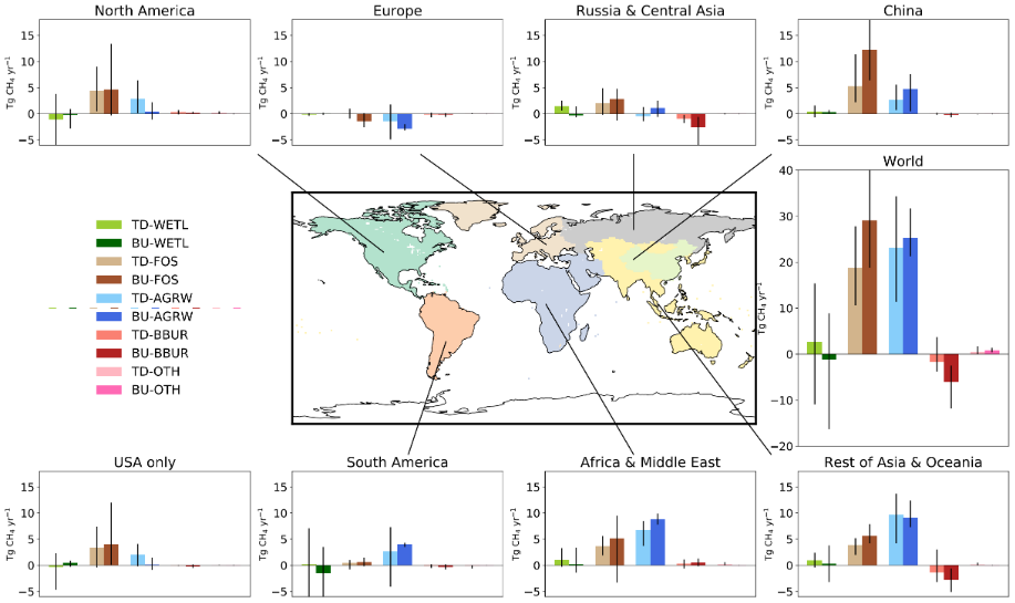
Fig. 8.30 A comparison of top-down (TD) and bottom-up (BU) methane flux measurements. Bars represent the difference between 2000-2006 emissions and 2017 emissions from wetlands (in green), fossil fuels (in brown), agriculture (in blue), biomass burning (in red) and ‘other’ (in pink). When the bar is positive, it means the emissions were greater in 2017 than they were in 2000-2006. In each case the top down estimate is given on the left and the bottom up estimate is given on the right. From Saunois et al., 2020.

When we summarise what we have learned about the methane cycle we see that the land surface is the largest emitter of methane, and that methane comes from a variety of sources, each of which has its own response to anthropogenic climate change. Unlike carbon dioxide, which is relatively ‘simple’ methane has natural sources and sinks that are themselves significant (~40%) and also are responding to warming temperatures. The methane budget is very difficult to quantify, and different techniques indicate different magnitudes of sources. And yet, due to its short lifetime, it is, and will remain to be, an easy target for emission reductions.