8.1. Plants, Soils and Eddies

We have touched on the importance of plants, vegetation, the land surface and soils, several times throughout the year.

• The land surface stores carbon from days, to years, to millennia

• Plants exert a biophysical control of evapotranspiration. Stomates (openings in plant leaves) control the interchange of water and \(\mathrm{CO_2}\) between the atmosphere and the plant. Think back to the groundwater lectures at the start of the year and the water balance equation.

• Momentum transfer - Plants create “friction” for the atmospheric flow near the surface. Plants create turbulent motions that enhance vertical mixing of heat and water vapor near the surface.

• Soil moisture availability - Plants have roots that determine the amount of water available for evapotranspiration. Soils more broadly control infiltration and thus influence the amount of flooding.

• Insulation - Plants that shade the surface and protect it from intense solar radiation and strong evaporation.

Plants also play a role in environmental temperature regulation. This was first conceptualised in a paper in 1983 by Watson and Lovelock, where they introduced the concept of Daisyworld. Daisyworld is a simple planetary model used to explore the effects of coupling between life and its environment. It is a nice analogue to how plant life grows and influences the environment around it. Daisyworld was, and is, controversial because it implies that planetary self-regulation can emerge from a series of realistic feedbacks without the need for organisms to adapt or change. Evolutionary biologists don’t really like it as a result. The paper is named “Biological homeostasis of the global environment: the parable of Daisyworld”.

Daisyworld

In this paper, Watson and Lovelock imagine a planet that is covered in two types of daisies, white daisies and black daisies, and land that has no daisies (gray soil). The daisies growth depends only on temperature, that is the assumption is that the soil has enough nutrients and everything else to support growth of the daisies. The further simplifying assumption is that there are no greenhouse gases, therefore the temperature of the planet is determined by solar luminosity and albedo, and albedo is impacted by whether the planet is covered in white daisies or black daisies.

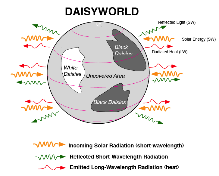
Fig. 8.1 A schematic of ‘DaisyWorld’.

If we consider the equation of population growth to describe the daisy fields:

(8.1)\[\pdv{\alpha}{t} = \alpha(p - \alpha) \beta(x) - \alpha \gamma(x) \]

Where \(\alpha\) is the fractional coverage of the ground by a species, \(p\) is the fraction of total habitable bare ground, and \(\beta\) and \(\gamma\) are the birth and death rates of the species, which depend on an environmental parameter \(x\). By convention \(p=1\) most of the time, but can be changed to represent there being some land that can’t be colonised by the daisies, e.g. ocean.

We can amend these equations for Daisyworld, for the ground covered by white daisies (\(\alpha_w\)) and the ground covered by black daisies (\(\alpha_b\))

(8.2)\[\begin{split}\pdv{\alpha_w}{t} &= \alpha_w(\alpha_g \beta(T_w) - \gamma) \\ \pdv{\alpha_b}{t} &= \alpha_b(\alpha_g \beta(T_b) - \gamma) \\\end{split}\]

Here \(a_g\) is the amount of available bare ground (\(\alpha_g = p - \alpha_b - \alpha_w\)) and \(T_w\) and \(T_b\) are the local temperatures felt by each daisy type (white and black, respectively). The death rate - \(\gamma\) - is kept fixed, and the functional form for \(\beta\) (the growth rate) is:

(8.3)\[\begin{split}\beta(T) = \begin{cases} 1 - k (T - T_{opt})^2 & |T - T_{opt}| < k^{-0.5} \\ 0 & \text{otherwise} \end{cases}\end{split}\]

Many people who have modelled Daisyworld have played around with \(k\), the width of the parabola, but in general people have settled on a \(k\) value so that the growth is bracketed between 5 and 40 °C.

The impact of the daisies on albedo is simple, white daisies have a fixed albedo (\(A\)) of 1 and reflect back all incoming light, while black daisies have an albedo of 0 and absorb all incoming light. Ground with no daisies is conventionally set to 0.5. Therefore the mean planetary albedo (\(A\)) is:

(8.4)\[A = \alpha_w A_w + \alpha_b A_b + \alpha_g A_g\]

The local temperatures that the daisies or bare ground feels, \(T_w\) and \(T_b\), which determines their growth rate, assumes linear diffusion of heat, and are given by

(8.5)\[\begin{split}T_w^4 = q (A - A_w) + T^4 \\ T_b^4 = q (A - A_b) + T^4 \\ T_g^4 = q (A - A_g) + T^4 \\\end{split}\]

Where \(T\) is the planetary temperature and \(q\) is a heat transfer coefficient. Finally the planet stays in thermal balance, as given by the 0D energy balance equation:

(8.6)\[S_o(1-A) = k_B T^4\]

Where \(S_o\) is the average solar energy incident on the surface of Daisyworld and \(k_B\) is the Stefan Boltzmann constant (5.67 x 10^-8 W m^-2 K^-4). The assumed value for \(q\) in the original paper is 2.06 x 10⁹ K⁴.

These equations make a system of multiple, non-linear feedback loops and the analytical solution is not simple. In the original paper, Watson and Lovelock solved the steady state solution, and many authors since have found analytical solutions to these equations. What is tested is a slowly rising solar constant, representing increased solar luminosity which drives increased temperature on Daisyworld. What happens then is that initially when the solar constant is still low, the black daisies grow preferentially to the white daisies, but as the solar constant gets stronger, the white daisies take over and grow relative to the black daisies. Eventually we reach temperatures that are too high and the white daisies all die too.

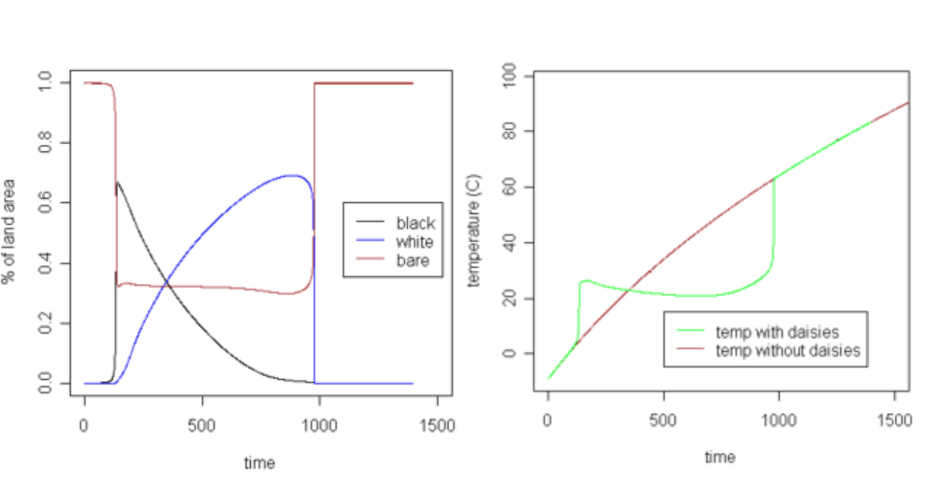
Fig. 8.2 Non-linear loops in ‘DaisyWorld’. Time is on the x-axis, but we can take time to be the stepped increase in solar luminosity.

What arises from these models is the fact that the presence of the daisies keeps the temperature of the planet equable at intermediate solar luminosity. This is the primary finding of Daisyworld, that the land surface, and particularly the types of plants on the surface, can evolve to adjust to help keep the global average surface temperature regulated. That is the parable of Daisyworld and allows us to motivate understanding what is on Earth’s land surface and the role that it plays in Earth’s climate and carbon system.

In addition to the plants on the surface, soils play a key role in Earth’s climate system. While the vegetation on land stores more carbon than the surface ocean, most (~80%) of this is in soils. As you may remember from the groundwater and flooding modules, soil type also controls infiltration and therefore plays a key role in our understanding of flooding and surface run off.

Soils

What are soils? Formally the definition is solid earth material that has been altered by physical, chemical and biological processes so that it can support rooted plant life. A mixture of organic matter, minerals, gases, liquids, and organisms that together support life.

Most people think of soils as the breakdown of plant material from above, and this does add to soils. However the majority of the soil, in terms of many of the key attributes like hydraulic conductivity and chemical content, is from the breakdown of rock material from below. The soil is a balance between the production from the erosion of the bedrock underneath and the erosion of the soil downslope.

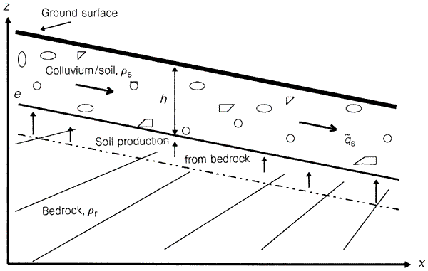
Fig. 8.3 A schematic of the formation of soil, which is a balance between the production from the erosion of the bedrock underneath and the erosion of the soil downslope.

The types of soil that are formed depend on many environmental factors, including Climate, Organisms, Parent Material, Topography and the amount of time the soil has to develop.

• Climate is key because it determines temperature and precipitation and the breakdown of the bedrock happens far more when there is more rain.

• The types of organisms also play a key role in the types of soils that develop – plants produce organic acids, and roots act to break apart the bedrock, they also help to stabilise soil profiles from run off and erosion. Indeed, rewilding is being used as flood mitigation measure in parts of the UK.

• The parent material is also key as different rocks breakdown differently, some breakdown completely and others breakdown partially and leave behind reactive particles.

  • Key to both of these are the metals available for life as well as the pH of the soil. Unlike the ocean, the pH in soils can range from 3.5 to 10, which impacts the redox mobility of various metals and therefore the microbial life that can be present. For example many key nutrients for plant life are pH sensitive. At neutral pH, only half the iron in soil is ‘bioavailable’, at low pH aluminium is at high concentrations and can be toxic, at high pH, calcium

• Topography is also key, as well as which direction the soil is facing, as it helps determine how thick the soil will be. Soils on hillslopes tend to be around 1 meter thick, while soils on flat surfaces can grow very thick.

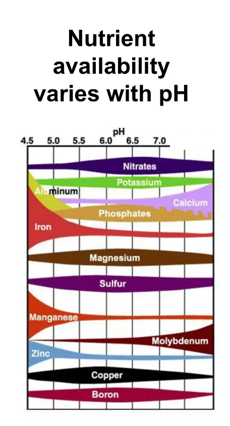
Fig. 8.4 The availability of nutrients in soil as a function of pH.

Soils end up representing the combined impact of additions to the ground surface, chemical reactions within the soil, vertical transfer and things that are removed, either eliminated through biology or chemistry or eroded away. They grow through the addition of organic matter (Fig. 8.4) and the weathering of rock (Fig. 8.5).

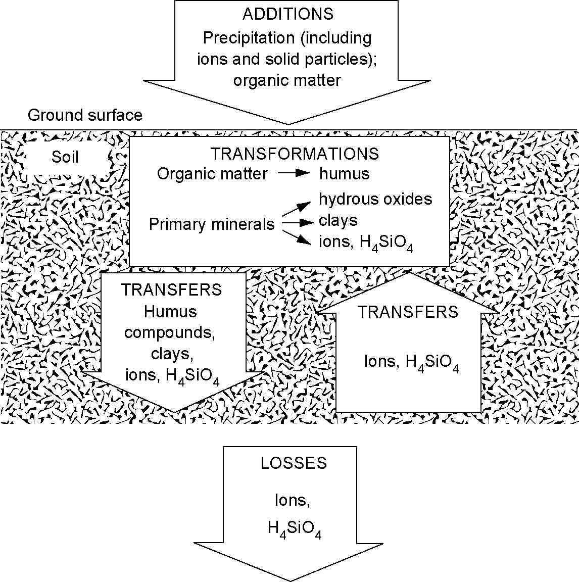
Fig. 8.5 Weathering processes that form soil.

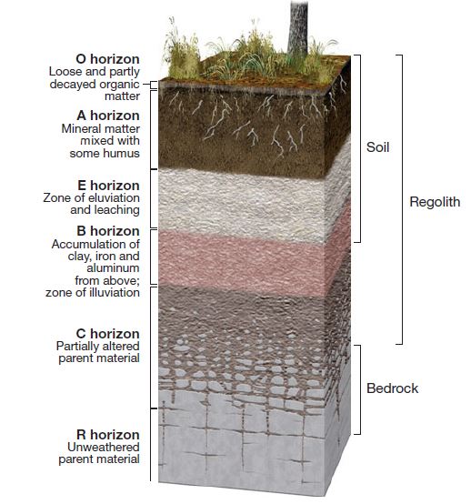
Fig. 8.6 Soil Horizons. Over time, soil layers differentiate into distinct ‘horizons’ which can be considered zones of chemical action.

• Chemical reactions and formation of secondary minerals (clays).

• Leaching by infiltrating water

• Deposition and accumulation of material leached from higher levels in the soil

If we link this back to the climate models we have been studying (and building) throughout this term, we can see that ultimately for a full climate model, we would need proper representation of the flow of mass, momentum, energy, and trace gases (e.g., water vapor, CO₂) between the surface and the atmosphere – soils and plants on the surface moderate this exchange. This has led to an entire class of models known as Surface, Vegetation, Atmospheric Transfer Models (SVAT).

Ultimately these models need to be parameterised by understanding exactly what controls soil moisture release, how much gas is coming off a forest or another ecosystem to feed into broader global climate models. This comes back to measurements you can make in the field. Throughout these lectures we will return to how measurements are actually made that help us understand what we put into global climate models.

In the case of understanding what is being released by plants and soils, one of the most common tools is to use a tower and use the Eddy Covariance technique to determine the gas or heat or moisture flux.

Eddy Covariance

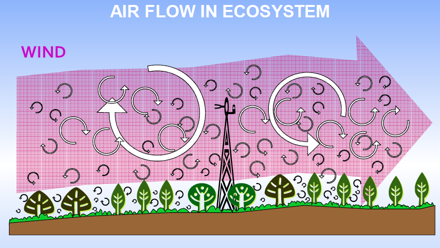
Fig. 8.7 The movement of air through ecosystems.

As we learned in the Global Environment lectures, air and water on our rotating planet are moved in turbulent eddies, which are like circular movements of fluid that serve to disperse and diffuse air particles and things in those air particles. These eddies have vertical and horizontal components.

• If we consider the vertical component, we see below that Eddy 1 moves parcel of air \(c_1\) down with a speed \(w_1\) while Eddy 2 moves parcel of air \(c_2\) up with speed \(w_2\).

• Each parcel of air has a concentration of some gas, a temperature, a water vapour content, if we know these and the speed \(w_x\) then we know the flux.

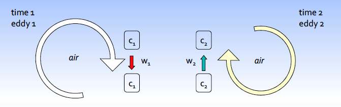
Fig. 8.8 A schematic of Eddy Covariance.

When we have turbulent flow, the vertical flux is equal to the mean product of air density (\(\rho_a\)), vertical wind speed (\(w\)) and the mixing ratio of the gas of interest (\(s\)).

\[F = \overline{\rho_a w s}\]

We consider this graphically below (Fig. 8.9). Properties in turbulent air parcels will fluctuate up and down because of wind gusts and movement of air. So we can consider both the average of a property below and the fluctuation above and below that mean.

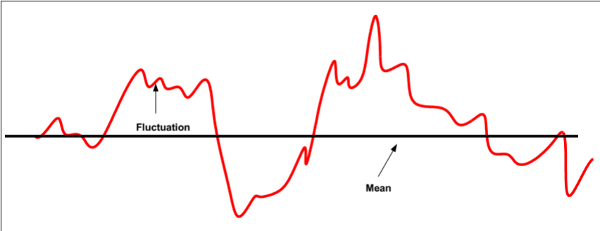
Fig. 8.9 The fluctuation of air around a mean driven by eddies.

We can use a technique called Reynolds decomposition to break the density, velocity and property of interest into the mean and the fluctuation around the mean.

(8.7)\[F = \overline{(\bar{\rho_a} + \rho_a') (\bar{w} + w') (\bar{s} + s')}\]

If we multiply this out and remove the terms with a single prime (because the average deviation around an average is zero, and make the assumption that there isn’t much variation in the density of air, and that there is no divergence or convergence in the flow, then the flux becomes

(8.8)\[F = \overline{(\bar{\rho_a} w' s')}\]

This means at any given instant, you can multiply velocity of air being moved upwards or downwards at a speed of m s^-1, by the fluctuation of the entity about its mean. If you average these you will get the net flux from the ecosystem. This gives you g of entity transferred vertically, per square meter of surface area per second.

Using this to get the carbon flux or the methane flux is relatively straightforward, you can make near instantaneous measurements of methane or \(\mathrm{CO_2}\) while also measuring the velocity of air and the average density of air. You can also use this to get the Latent Heat emitted from the surface, as well as the Sensible Heat (remember from Michaelmas that these are two of the key ways that the Earth re-radiates heat. In the equation below we derive the sensible heat flux by multiplying the average air density with the instantaneous velocity and temperature and convert it to energy units with the specific heat capacity of water.

\[Q H = \bar{\rho_a} C_p \bar{w'} \bar{T'}\]

The advantages of Eddy Covariance are

• Averages small-scale variability of fluxes over a surface area that increases with measurement height

• Measurements are continuous and in high temporal resolution

• Fluxes are determined without disturbing the surface being monitored

• Great tool to look at ecosystem physiology

The disadvantages are

• Need turbulence!

• Gap filling issues

• Relatively Expensive

• Stationarity issues

• The eddy covariance method is most accurate when the atmospheric conditions (wind, temperature, humidity, \(\mathrm{CO_2}\)) are steady, the underlying vegetation is homogeneous and it is situated on flat terrain for an extended distance upwind.