6.5. Atmospheric heat transport#
In this section, we will describe the mechanisms leading to poleward heat transport in the atmosphere and develop a simple model to predict the equilibrium temperature distribution. While the mean meridional circulation in the atmosphere (e.g. the Hadley circulation) is capable of transporting heat, most of the heat transport in the atmosphere is associated with transient features.
The thermal wind balance introduced in the previous section is a state of equilibrium; the force exerted by the hydrostatic pressure gradient is balanced by the Coriolis acceleration. This equilibrium is unstable. Imagine starting with an east/west jet in thermal wind balance with the mean temperature gradient. Because the wind is in a state of equilibrium, it will be steady (\(\partial \mathbf{u}/\partial t=\mathbf{0}\)). However, because the equilibrium is unstable, if we give this perturb this equilibrium state by a small amount, the perturbation will grow. As a result, the east/west jet will develop meanders, some of which will eventually develop into closed eddies. These are the weather systems that bring us periods of wet and dry weather.
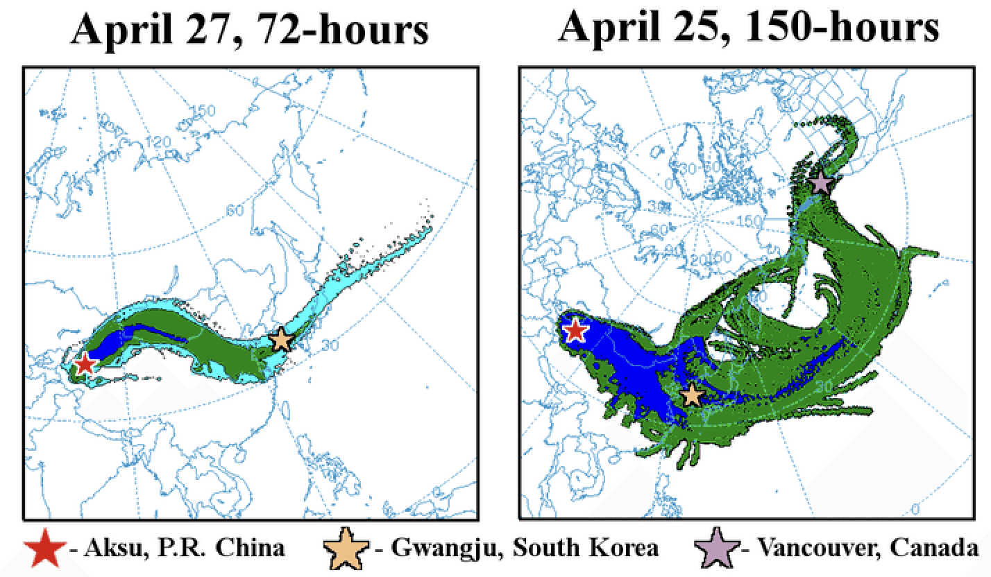
Fig. 6.16 Trajectories of dust particles originating in western China (Cottle et al. 2013).#
As air parcels are transported by meandering jets and eddies, they trace out chaotic trajectories. For example, Fig. 6.16 shows trajectories of small dust particles from a source in western China, inferred from a forecast model. Notice how the collection of particles spreads out as they travel to the east. This process is important for dispersing dust, aerosols, and pollutants. The chaotic motion induced by transient eddies also transports heat from the equator towards the poles.
Our goal in this section is to build a mathematical model for the temperature of the atmosphere as a function of latitude and time. Since we will be relating changes in temperature to heat, we need to introduce the heat capacity of the atmosphere, \(C_a\). Changes in heat, \(\Delta Q\), are then related to changes in temperature, \(\Delta T\) according to \(\Delta Q=C_a \Delta T\).
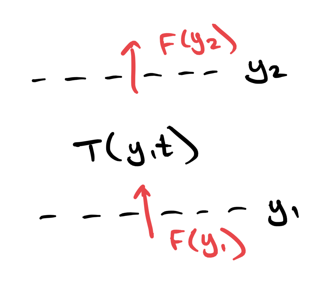
Fig. 6.17 Sketch of a control volume in the atmosphere with mean temperature \(T\) and heat fluxes \(F\).#
Consider the time rate of change in the temperature of the atmosphere, averaged in a control volume with a line of constant latitude, \(y=y_1\), on its southern boundary and \(y=y_2\) on its northern boundary as sketched in Figure Fig. 6.17. We can think of the average temperature in the control volume, \(T\), as being averaged around the globe for all longitudes and averaged in height. A northward heat flux through the southern boundary of our control volume, \(F(y_1)>0\) will cause the temperature in our control voluem to increase. Similarly, a northward heat flux through the northern boundary of our control volume, \(F(y_2)>0\), will cause \(T\) to decrease. Since the heat is being spread over a distance \(\Delta y=y_2-y_1\), we have that
If we factor out a minus sign from the right hand side and let \(\Delta y\rightarrow 0\), then this equation becomes
Next, we need to model the heat flux. We expect heat to flow from warm regions (near the equator) to cold regions (near the poles). We will further assume that the heat flux is proportional to the local north/south gradient in temperature:
where \(\kappa\) is the constant of proportionality. Note that the minus sign is needed since we will take \(\kappa\) to be positive and if the temperature is decreasing to the north (as in the Northern Hemisphere), we expect heat to flow to the north. Using this form for the heat flux in Eq. (6.18) gives
This is the so-called diffusion equation which we have seen previously in the context of contaminents moving through groundwater and heat conducting through ice. In the context of the atmosphere, we also want to add heat fluxes associated with incoming solar radiation and heat radiating back to space. Specifically, we will let \(I\) represent the net incoming shortwave radiation and \(O\) represent the outgoing longwave radiation. We will assume that \(I\) is a function of latitude, while \(O\) is a function of temperature (since warm objects radiate more heat than cold objects). Adding these additional heat sources to Eq. (6.20) gives
Let’s breifly discuss the units involved in Eq. (6.21). Here, we will let \(y\) be the distance (in meters) measured north from the Equator[1] and \(t\) is the time in seconds. By comparing the first and last terms, we can deduce that the units of \(\kappa\) must be L\(^2\)/T. The units of \(I\) and \(O\) are in \(\mbox{W}/\mbox{m}^2\), and \(C_a\) is the heat capcity of a vertical column of atmosphere per unit area. Recall that the heat capacity of air is about 1000 J/kg/\(^\circ\) C and the mass of the atmosphere is about \(10^4\) kg/m\(^2\). Therefore, \(C_a\simeq 10^7\) J/m\(^2\)/\(^\circ\)C.
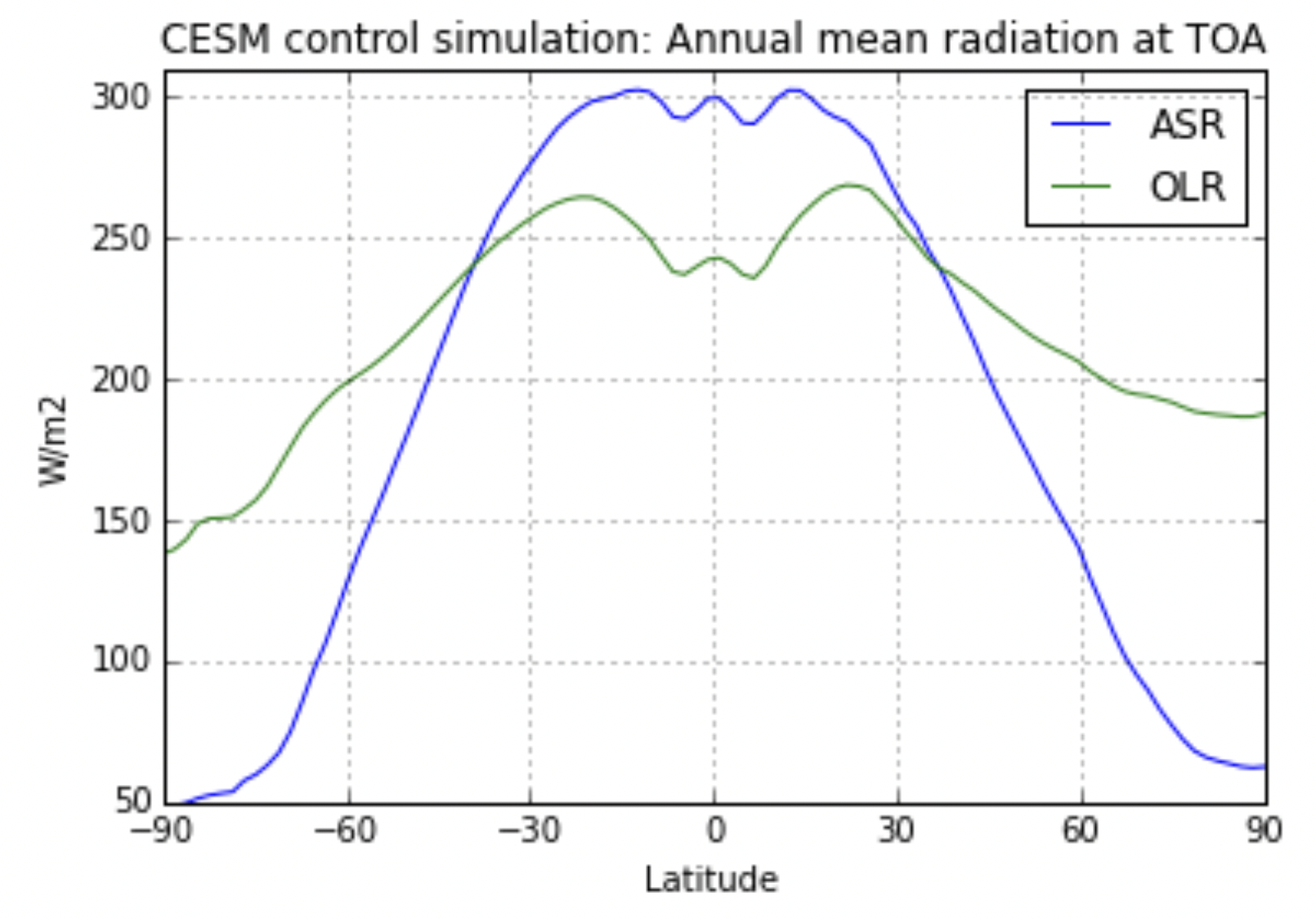
Fig. 6.18 Net incoming shortwave (ASR) and outgoing longwave (OLR) radiative fluxes at the top of the atmosphere.#
Fig. 6.18 shows profiles of the incoming shortwave and outgoing longwave radiative fluxes at the top of the atmosphere. Here, we we assume that the incoming shortwave flux is a function of latitude only. Inspired by Fig. Fig. 6.18, we could take
where \(R_e\) is the radius of the Earth and \(Q_{max}\) is the maximum incoming solar radiation (which occurs at the equator (\(y=0\))). The argument to the \(\cos\) function is set so that this term vanishes at the poles where \(y=\pm \pi R_e/2\). Based on Fig. 6.18, the difference between the incoming shortwave radiation at the equator and poles is about 250 W/m\(^2\), so we take \(C=125\) W/\(m^2\). The global average of the incoming shortwave radiation is about 240 W/m\(^2\), so we take \(D=115\) W/m\(^2\). Note from comparison with Fig. Fig. 6.18 that this value makes the incoming shorwave radiation too high, but this is needed to yield the correct mean value while accounting for the fact that the equatorial region has a larger surface area per degree latitude than the polar regions. We could also include time-dependence in \(I\) to represent seasons, but here \(I\) instead represents an idealized annual average.
Recall from the atmospheric chemistry lectures that the outgoing longwave radiation depends on the atmospheric temperature. It is important to account for this if we want to create a model that is capable of capturing climate states that are different to the one that we are currently experiencing. A simple way to represent the temperature dependence on the outgoing longwave radiation is using a linear function:
Reasonable values for the constants are \(A=210 \mbox{W}/\mbox{m}^2\) and \(B=2 \mbox{W}/\mbox{m}^2/^\circ \mbox{C}\).
Combining these terms, Eq. (6.21) becomes
Now, let’s consider the possible steady state solutions to Eq. (6.22). We will refer to the steady state temperature as the equilibrium temperature, \(T_e\). Since we are removing the time dependence, \(T_e\) depends only on latitude and hence the equation changes from a partial differential equation for \(T(y,t)\) to an ordinary differential equation for \(T_e(y)\): Eq. (6.21) becomes
Since this is a second order ODE, we need two boundary conditions. One choice is to ensure that the heat flux vanishes at the poles which requires that
Based on this boundary condition and the form of Eq. (6.23), we might guess that the solution will be of the form
Notice that this form for \(T_e\) always satsfies our boundary conditions. All that is left is to plug it into Eq. (6.23) and find \(\alpha\) and \(\beta\). After re-arranging terms, we have
Since this equation must hold for all values of \(y\) (including \(y=90^\circ\) where \(\cos{y}=0\)), the terms in both sets of parentheses must both vanish. Hence, we find that
From Eq. (6.24), we see that the equator to pole temperature difference is proportional to \(\beta\). When \(\kappa\) increases, \(\beta\) will decrease, consistent with our intuition above that diffusion will tend to make the temperature more uniform.
In order to estimate the equilibrium temperature distribution, we still need to specify the diffusivity, \(\kappa\), the units of which are L\(^2\)/T. We can estimate \(\kappa\) as the product of characteristic velocity and length scales, \(\kappa=U*L\). A typical wind speed associated with weather systems in the troposhere is \(U\sim 5\mbox{m}/\mbox{s}\), while a typical eddy size is \(L\sim 1000\mbox{km}\). Hence a reasonable value is \(\kappa \sim 5\times 10^6 \mbox{m}^2/\mbox{s}\).
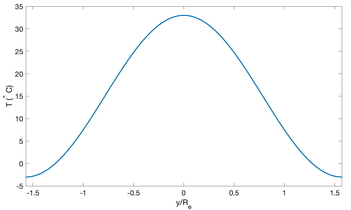
Fig. 6.19 Equilibrium atmospheric temperature distribution from the diffusive model in Eq. (6.22).#
From the estimates above, we have \(\alpha\simeq 15^\circ C\) and \(\beta\simeq 18^\circ C\). Fig. 6.19 shows the equilibrium temperature from Eq. (6.24) with these constants. Comparing this with the Earth’s mean temperature in Fig. Fig. 6.2, the diffusive model gives a reasonable equilibrium temperature distribution.