10.2. Solar Power#
Solar power is generated from the incoming solar radiation which reaches the Earth surface. At the edge of the atmosphere the solar radiation is about 1.361 kW m-2. As it passes through the atmosphere, it meets clouds, vapour, aerosols and some becomes scattered leaving about 1 kW m-2 to reach the surface. At any instant, the projected surface area is about \(pR^2\) where \(R\) is the radius of the Earth and so with an approximate radius of 6700km, this leads to an incoming radiation with energy flux order 1.4×10¹⁷ W (1.4×10⁸ GW).
The world uses 1.8×10⁴ GW of power, so the solar radiation is about 10,000 times greater than we need for all our power but it needs to be collected and distributed.
Solar photovoltaics (PVs) and parabolic solar collectors both provide a solution to achieve this and solar photovoltaics are now highly commoditised and they represent the largest part of the world’s installed solar energy generation. Silicon PVs are now cheap and widespread. When a photon with sufficient energy is absorbed, an electron can be emitted from the outermost shell, producing an electron-hole and therefore a current; the band gap required to do this is fixed at about 1.1 eV. The excess energy of the photon may be converted to heat. Shockely and Queisser have established that a single junction cell has an efficiency maximum of about 34%, so only 34% of the incoming radiation can be converted to electricity. However, in practice, most commercial cells are in the range of about 18-23%.
Research into photovoltaic cells is achieving progressively more efficiency in the laboratory setting (Fig. 10.13) but translation into the market, and resourcing the materials can lead to challenges/time delays in realising such performance in commercial scale products.
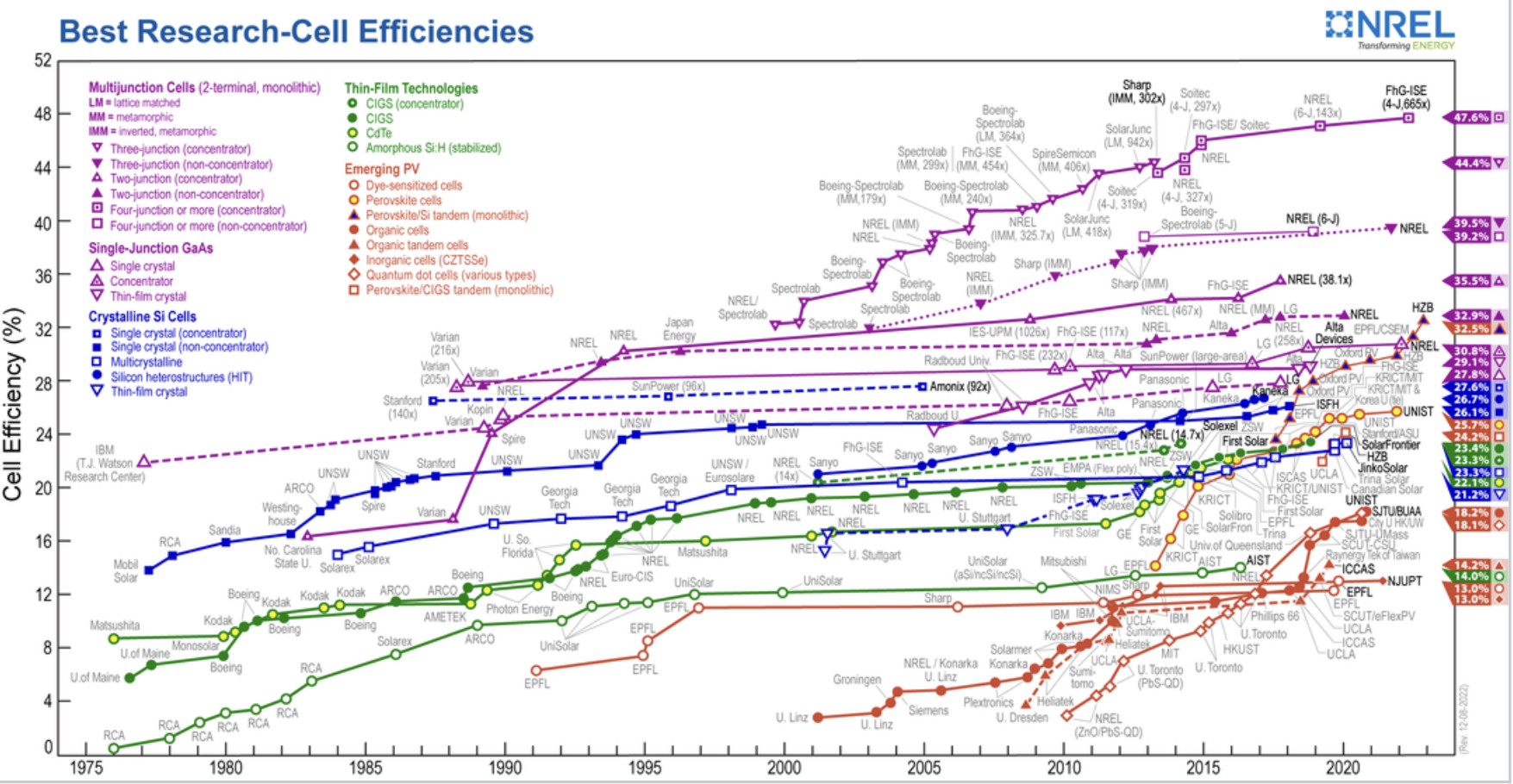
Fig. 10.13 Reported timeline of research solar cell energy conversion efficiencies since 1976 (National Renewable Energy Laboratory, USA). The panels convert visible light and shorter wavelength radiation, and can generate about 20% of the incoming radiation.#
The local environment has an important influence on the magnitude of this incoming radiation, as well as the location of the PV relative to the equator. Fig. 10.14 illustrates the mean annual radiation across the globe.
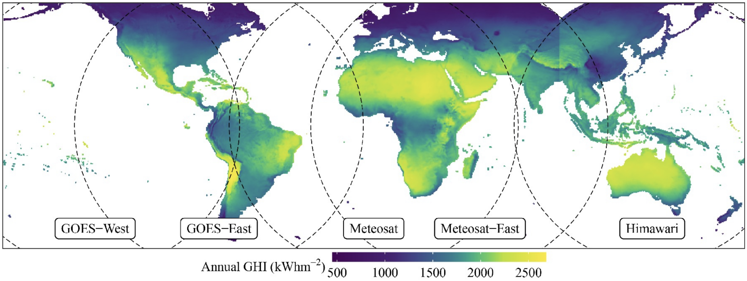
Fig. 10.14 Five geostationary weather satellites jointly cover all locations on Earth between ±60° latitude. Gridded irradiance estimates can be derived from the visible- and infrared-channel images captured by these satellites. Other meterological satellite series, such as Fengyun, are not shown, since their field-of-views overlap with the ones in the figure. Data source: National Solar Radiation Database.#
It is seen that very high radiation energy exists near the tropics but in the equator region it falls off a little, as it does at more northerly and southerly latitudes. This is a result of vapour near the equator which scatters some of the radiation, leading to less direct radiation reaching the surface. As we move towards the poles, the light is passing through more atmosphere and so suffers more attenuation.
If we are to model the power which can be generated by a PV panel, we require details of this incoming direct radiation, and also the diffuse radiation which is created as a result of the scattering. We also require knowledge of the variation of the radiation over each day as the Sun rises and sets, and over the seasons as the length of day increases. The more time the Sun is higher in the sky, the more the intensity of the radiation increases.
Daily and Seasonal Fluctuations#
Fig. 10.15 illustrates the mean daily irradiation on the Earth’s surface in MJ m-2 across the UK for January and July. The colour mapping of the two figures is different owing to the very different levels of radiation. In winter, the UK get about 2.5-3 MJ/m-2 at best in the southern most part of England while the July data shows an increase to about 19-21 MJ m-2, nearly a factor of 6-7 larger. We also see a very large gradient between southern England and northern Scotland.
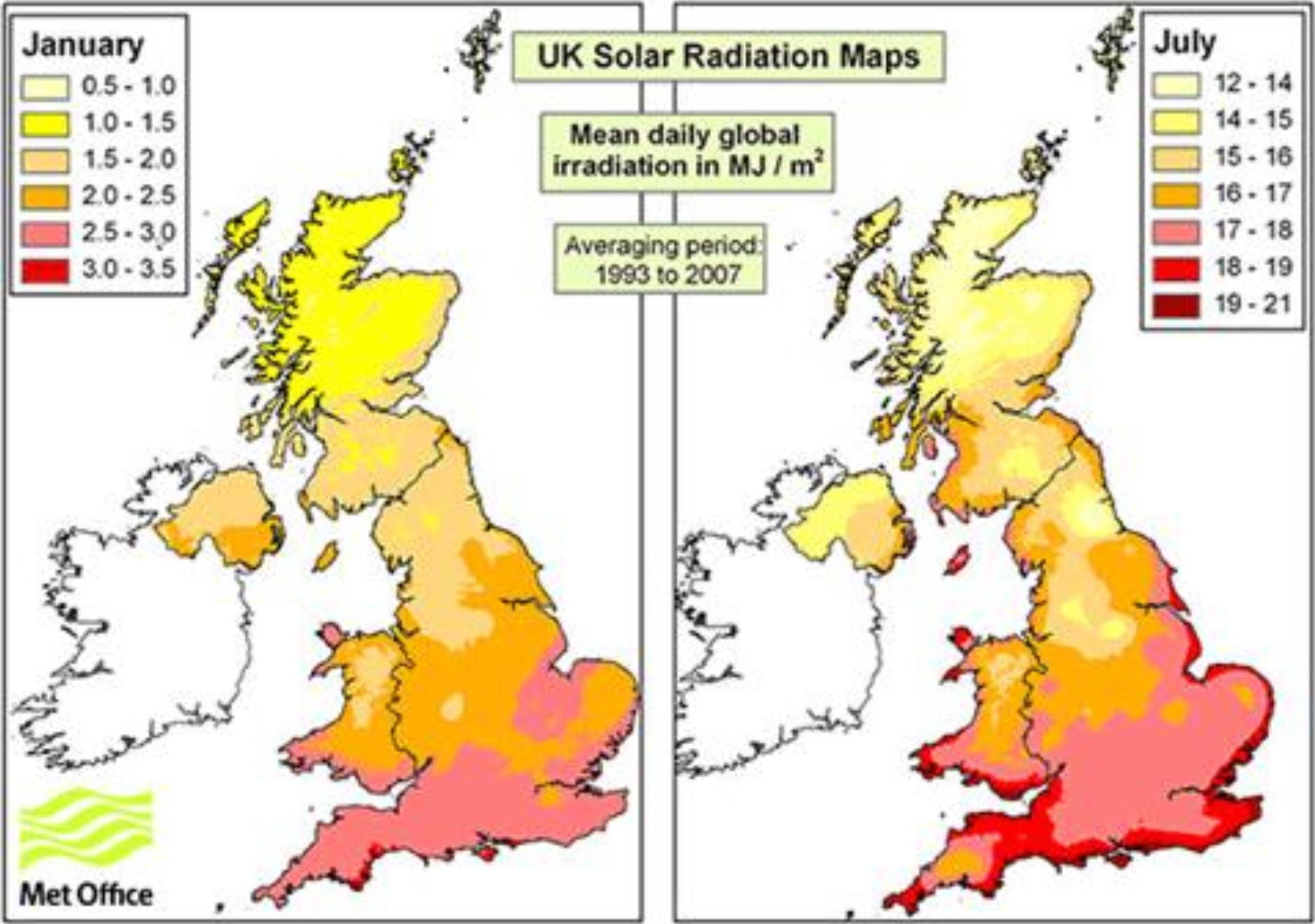
Fig. 10.15 Solar insolation maps for the UK in January (left) and July (right). They show the average daily irradiation levels for all areas of the UK for January and July. Note how the level of irradiation is as much as 10 times greater in July than it is in January.#
On a given day, the radiation increases rapidly after sunrise, reaches a maximum then decreases again (Fig. 10.16). This pattern applies throughout the seasons, but with a longer period of light and larger maximum radiation on the surface as we move from winter to summer.
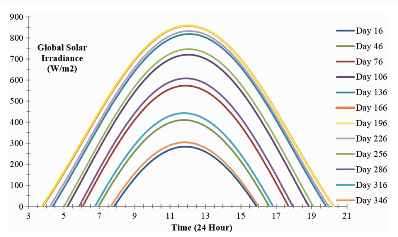
Fig. 10.16 Variation in radiation with time over a series of days, starting with New Years day as day 0.#
This power vs. time relation means there are challenges for PVs as an energy source for the electricity grid, as it requires stable power supply. So in the evening as the Sun drops, other energy sources are needed. In California, there is now so much solar power that when the solar power drops out, the alternative sources need to come online extremely quickly to cover demand (Fig. 10.17).
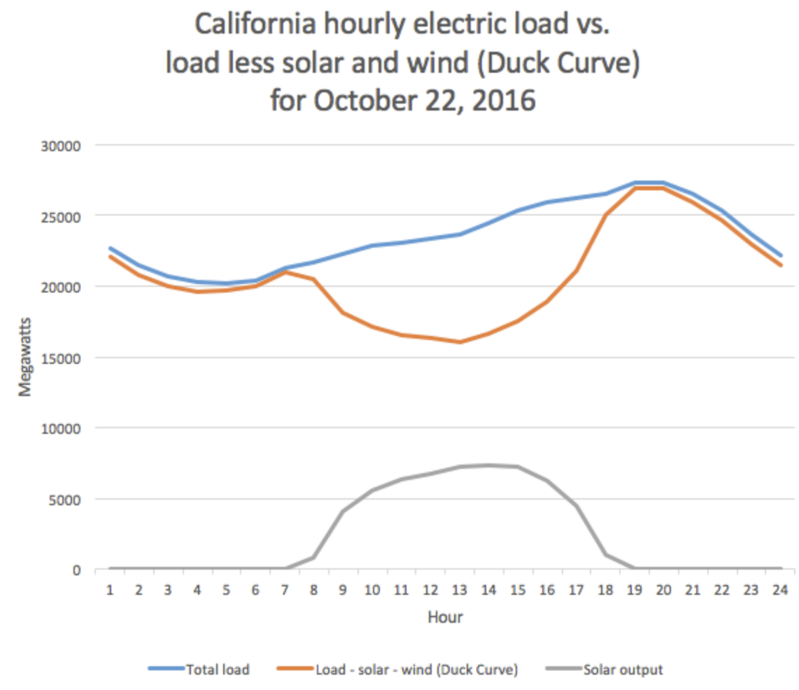
Fig. 10.17 The difference between total electric load and renewable power. When solar power drops out, the alternative sources need to come onstream extremely quickly to make up the deficit.#
In order to calculate the power produced by a PV cell, we can combine this incident radiation data over a year with the efficiency and capacity of the PV cell: this is a key parameter in the design of solar installations. However, the above model for the irradiance (Fig. 10.16) derives from predictions of the magnitude of both the direct and diffuse radiation (Fig. 10.18). On a clear day, the direct radiation represents about 85% of the signal, with the other 15% being diffuse. In contrast on either a cloudy or polluted day with, for example, smog, the direct radiation may be very small and most radiation reaching the Earth’s surface will be diffuse. Modelling and predicting this partitioning of the radiation is key for predicting the performance of a PV cell, and as the fraction of solar power in the energy system increases, the accuracy of such predictions will be key for managing the resource.
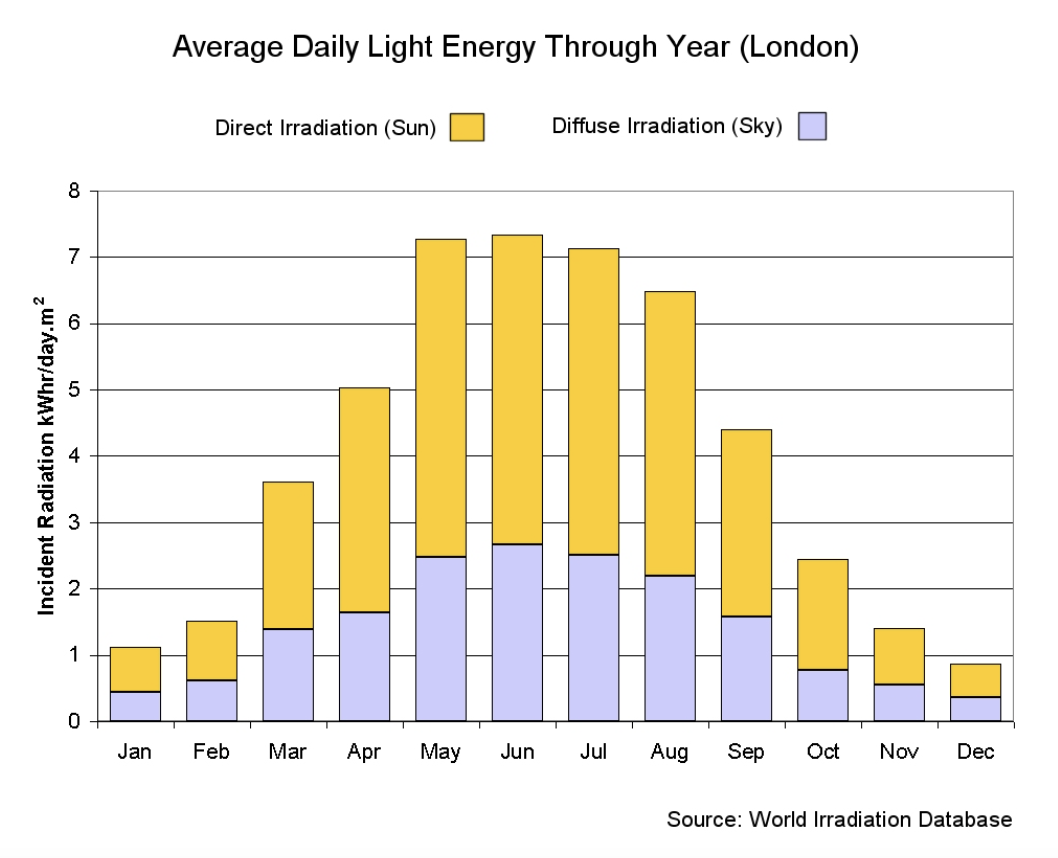
Fig. 10.18 The partitioning of direct and diffuse radiation in London.#
It is seen that a good part of the radiation is diffuse, on average, owing to the often overcast weather conditions. Also because London is quite far North, the summer and winter radiation is very different. In contrast, if we look at somewhere hot and arid like Aden, the summer radiation is only 30% diffuse, with total value 7 kWh m-2 and the winter is 35% diffuse with about 5.25 kWh m-2 solar radiation, a much smaller change.
In detail on a given day, the actual incident radiation fluctuates owing to the intermittency of the cloud cover (Fig. 10.19). In terms of supplying a constant source of energy, these high frequency fluctuations mean that a large high frequency storage is needed to smooth out the supply.
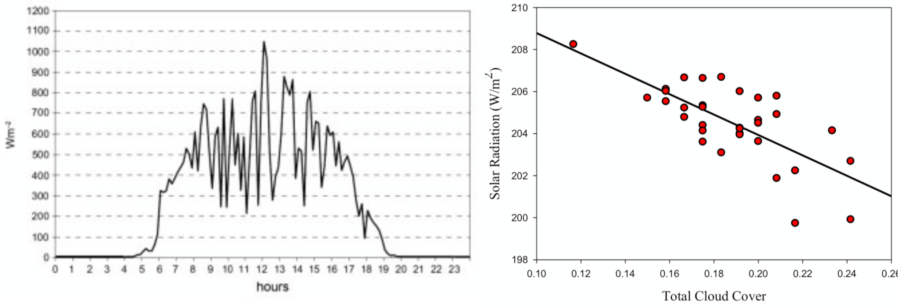
Fig. 10.19 Influence of the extent and genera of cloud cover on solar radiation intensity.#
Data on the impact of cloud cover on the total incident radiation suggests a trend of decreasing radiation with cloud cover, but there is also scatter owing to additional factors.
Panel orientation#
A second issue which influences the power output of a panel is the direction to the horizontal which the panels take. As the Sun moves round the sky during the day, and as its position in the sky varies seasonally, a fixed panel not remain normal to the radiation, and this decreases the power generated. Some panels do have a control to enable variable angles, but otherwise a fixed panel has an optimal angel when averaged over the year’s power production. In the UK this is about 35 degrees to the horizontal (Fig. 10.20). This is generated as a geometric calculation, following the position of the Sun with time relative to the panel.
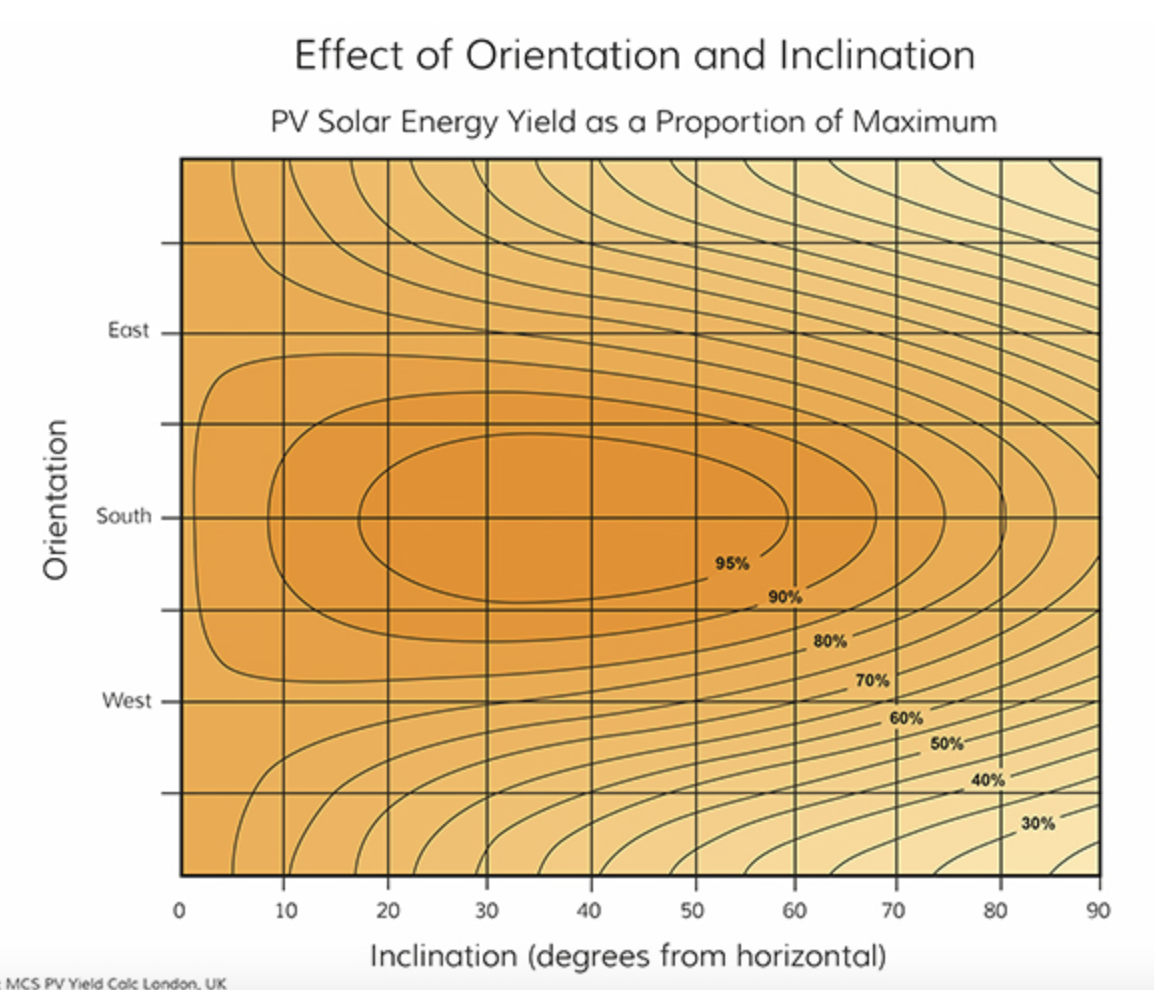
Fig. 10.20 Contour plot illustrating the drop off in total production with other angle of tilt.#
Climate trends#
It is of interest to record the change in cloud cover over Europe and the associated change in surface radiation over the past 35 years, since the data show a trend of decreasing cloud cover and increasing radiative flux. This change is a few percent of the total.
Storage#
If the incoming radiation on a particular day has the idealised form
where
then the average power over a day, \(\bar{P}\), of length \(T\), which can be collected with a panel of efficiency \(E\) is found by integrating \(P\) with respect to time, \(t\), leading to
We can also calculate the amount of energy which we would need to store in order to supply this average power output to the grid constantly. We would do this by storing excess energy at times when the power output was above average, and supply it back to the grid when output was below average. If \(t_1\) and \(t_2\) are the times when the instantaneous power output, \(EP(t)\), matches the average power \(\bar{P}\), then the amount of energy storage, \(S\), required is
Over the seasons, \(A\) will change from winter to summer, and \((t_{set} – t_{rise})\) also becomes longer, and so the power stored increases nonlinearly with the season. We will now turn to understanding this storage in more detail, as there is both diurnal storage and interseasonal storage required (Fig. 10.21).
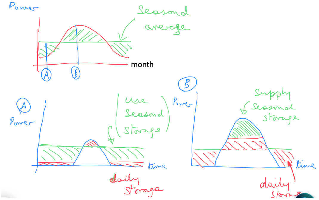
Fig. 10.21 A schematic of the annual variation in solar radiation and the storage required to smooth out the power output.#