4.6. Flooding

Overtopping the bank

A river flowing through the landscape may overtop its embankment, as shown in Fig. 4.23. The means water flows out of the channel and inundates the surrounding flood plane, and eventually can reach towns and other urban areas.

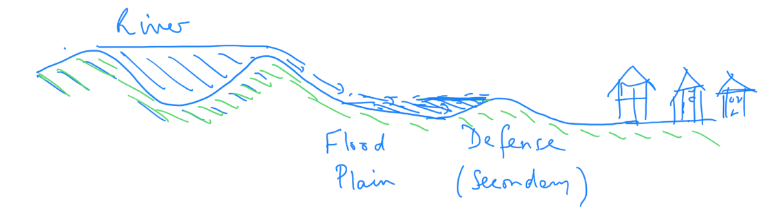
Fig. 4.23 A river overtopping its banks and flowing on to the flood plain.

We wish to determine the rate at which water is flowing out of the river. The situation is shown in more detail in Fig. 4.24.

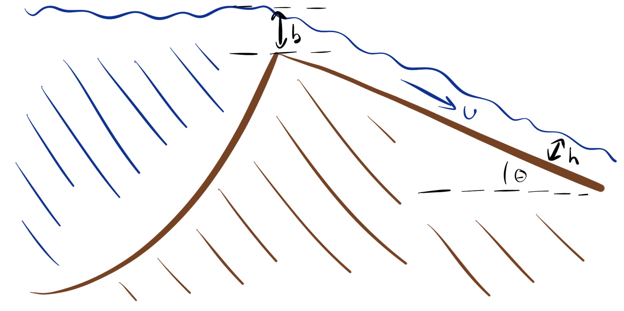
Fig. 4.24 A river overtopping its banks and flowing on to the flood plain.

The flow rate of the water moving over the embankment depends on the velocity of the water flow and the height over the top of the bank, \(b\). If the speed of the water is \(\sim \sqrt{gb}\) (as discussed in Section 4.3) then the flow rate per unit length along the embankment goes as

\[Q \sim \beta b \sqrt{g b}\]

where \(\beta\) is a geometric factor of \(\frac{2}{3\sqrt{3}}\) in the idealised case. With the flux over the bank established, we can turn our attention to the flow down the slope, further away from the levee.

Balancing the flows in and out of a control volume in the flow, as we have previously, we get a differential equation describing the rate of change of the thickness of the flow, \(h\):

(4.25)\[\pdv{h}{t} = -\pdv{Q}{x} + I\]

where \(I\) is an infiltration term. With rapid flow from the river, the flow is turbulent in the flooding zone, and the speed of the flooding water is given by

(4.26)\[u = \sqrt{\frac{gh \sin{\theta}}{C_D}}\]

and we can substitute into (4.25) using \(\pdv{Q}{x} = \pdv{(uh)}{x}\):

\[\pdv{h}{t} + \frac{3}{2} \sqrt{\frac{g \sin(\theta)}{C_D}} h^\frac{1}{2} \pdv{h}{x} - I = 0\]

So taking the steady state condition, \(\pdv{h}{t} = 0\) and integrating we get

\[h(x)^\frac{3}{2} - h(0)^\frac{3}{2} = - \sqrt{\frac{C_D}{g \sin(\theta)}} I x\]

and so we can see that \(h(x) \rightarrow 0\) when \(x \rightarrow \sqrt{\frac{C_D}{g \sin(\theta)}} \frac{h(0)^\frac{3}{2}}{I}\). \(I\) is small when the ground is waterlogged, and so \(x\) gets large, which holds with our general intuition about flooding.

With this model we can then assess how long the flood plain next to a river will take to fill up with water. If there is a secondary defence before the flood reaches the town along the river, as in the sketch, this flood plain provides a buffer to protect the town.

Non-examinable: derivation of \(\beta\)

If waters flood from a river, over the embankment, the flow rate of the water moving over the embankment depends on the height of the water in the centre of the river compared to the height at the embankment. If the water level decreases by an amount \(h\), the flow speed over the embankment is \(\sqrt{(gh)}\) and if the depth of the water is \(b\) at the embankment, the total flux is

\[Q = b(g h)^{1/2}\]

per unit length along the embankment. The height of the embankment below the height of the free surface of the river in the centre of the river above the river bed, \(H\), can be written as \(H-(b+h)\). At the crest of the embankment, the height above the base of the river is a maximum, and so if \(y\) is the coordinate normal to the river, then

(4.27)\[\dv{h}{y} + \dv{b}{y} = 0\]

If we differentiate the expression for the flux \(Q\) above with respect to \(y\), then the answer should be zero (as the flux is constant in space) and using Eq. (4.27) we then find that

\[2h = b\]

and so

\[3 h = (H_r - H_e)\]

Where \(H_r\) and \(H_e\) are the heights of the water surface in the centre of the river and the top of the embankment above the base of the river. This leads to the result that the flux is given by

\[Q = \frac{2}{3 \sqrt{3}} g^{1/2} (H_r - H_e) ^{3/2}\]

Where we can see we have approximated \((H_r - H_e) \sim b\) in the formula we used in the lectures.

Flood defense barriers

A flood defence barrier needs to withstand the pressure from the flood water. This leads to a horizontal force on the barrier which can be calculated from the integral of the hydrostatic pressure on the wall of the barrier.

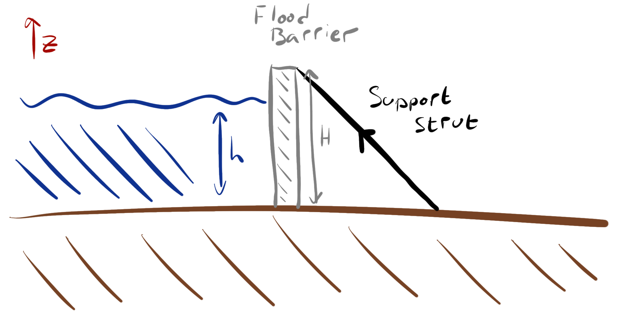
Fig. 4.25 A flood defence barrier, height \(H\), holding back water at a height \(h\).

Since the atmospheric pressure acts on both sides of the barrier, we can ignore it. Therefore, the net pressure acting at a point on the barrier as a function of \(z\) is

\[P(z) = \rho g (h-z)\]

and the total force acting will be

\[F = \int_0^h P(z) dz = \frac{\rho g h}{2}\]

A torque will also act on the barrier, which will be of the form

\[F = \int_0^h z P(z) dz\]

To prevent the barrier rolling over there needs to be a system to withstand this torque, which may include a series of inclined support rods pressing on the top of the barrier from the ground on the non—wet side of the barrier.

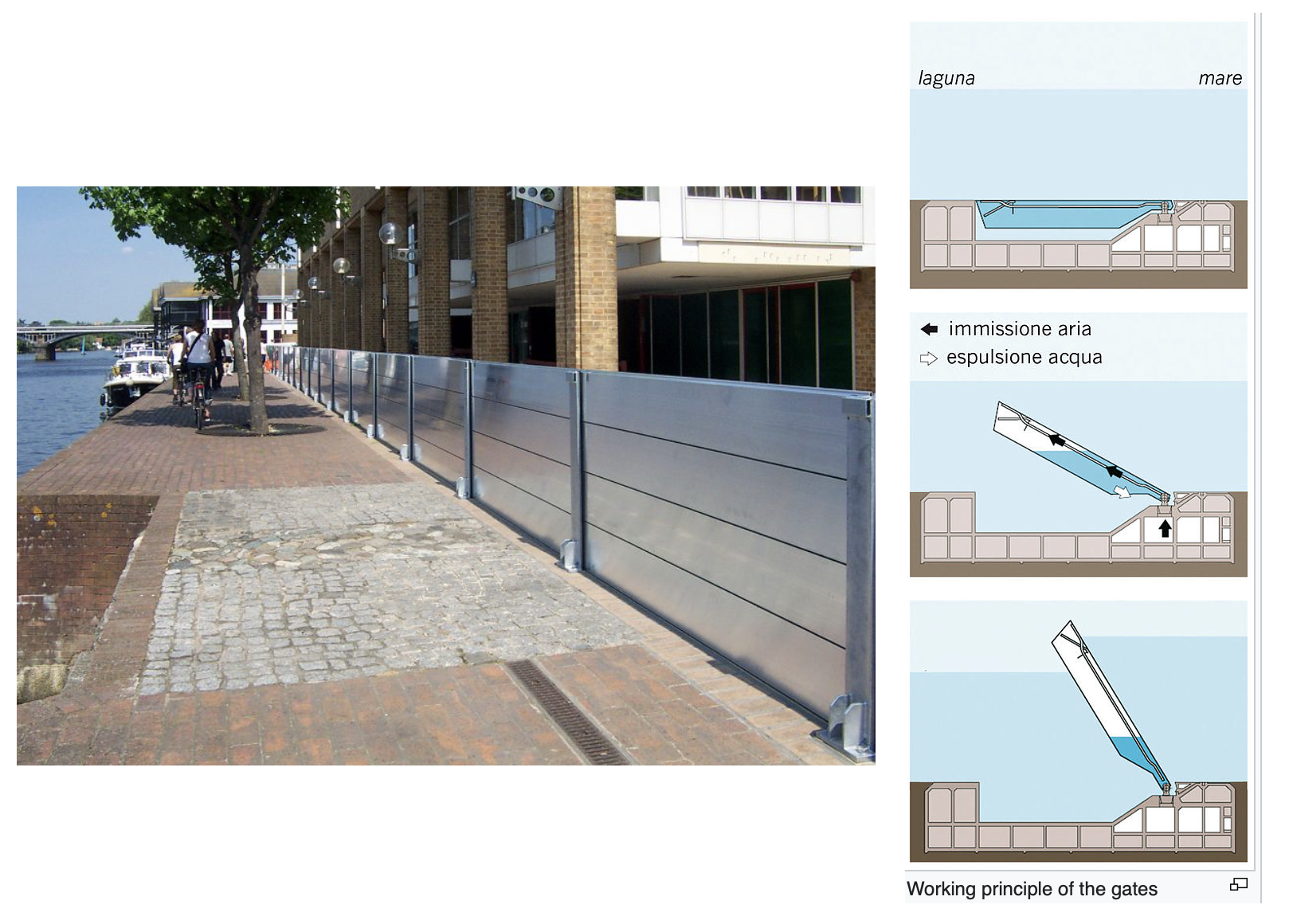
Fig. 4.26 In the Venice lagoon there are some interesting flood barriers which float up to the surface to stop incoming flow as in the figure above from the MODA website.

Objects carried by a flood

A particular challenge in a city environment for a flood relates to the transport of debris by a flood. Cars, logs and other large objects can be swept downstream and lead to blockages and the build up of very large forces by continuing floodwaters and damage.

There are several key elements to assessing the transport of an object by the flood which makes for an interesting calculation. For example, a static car without any flood water has a weight \(Mg\) balanced by an upward normal force \(N = Mg\). The sliding friction is typically given by a fraction \(\mu\) of this normal force, and so the critical force needed to move a dry car would be \(\mu Mg\).

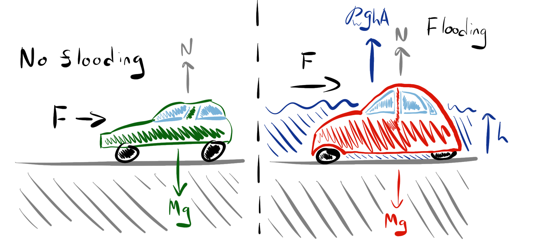
Fig. 4.27 The ability of a car to resist movement.

In a flood, if the car is submerged to a depth \(h\), and the car is waterproof then, modelling the car as a cuboid with a basal area \(A\), we find there is an upward buoyancy force, \(F_B\), from the water pressure acting on the base of the car given by

\[F_B = \rho g h A\]

Hence, the upward normal force from the ground is reduced and is now given by

\[N = M g - F_B\]

The horizontal force needed to move the car is now \(\mu (Mg – F_B)\) assuming that the coefficient of static friction is the same irrespective of the presence of the water. So, it is easier to move the car owing to the buoyancy from the presence of the water.

If the water flowing around the car has speed \(u\), then the force on the car will be

\[F = C_D \rho u^2 W h\]

where the width of the car is \(W\) and the water depth is \(h\) and \(C_D\) is the drag coefficient for the water flow round the car.

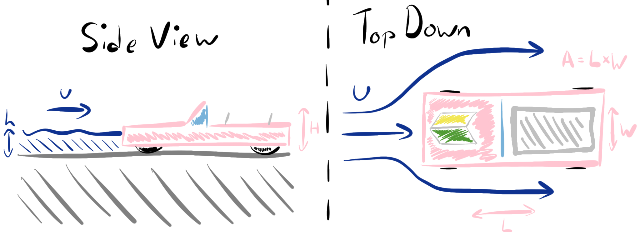
Fig. 4.28 Forces exerted on a car in a flood.

This leads to the result that the water speed required to move the car depends on the depth of the water according to the relation

\[C_D \rho u^2 W H = \mu (M g - \rho g h A)\]

Since \(M = AH \rho_c\) where \(\rho_c\) is the density of the car and \(H\) and height of the car (the bulk density, which is about \(0.4-0.5 \mathrm{kg~m^3}\)) then with \(\mu = 0.2\), \(h = 0.5 \mathrm{m}\), \(A=3 \ \mathrm{m^2}\) and \(H = 1 \ \mathrm{m}\), we find the critical \(u\) has value of about \(1-2 \ \mathrm{m~s^{-1}}\).

If \(h\) increases towards \(0.5 \mathrm{m}\), then the buoyancy force is much greater, and the car is on the edge of floating off, so the drag force and hence current speed required to move the car falls to much smaller values.

Flooding through a city

When a flood passes through a city, the advance of the flood may be strongly controlled by the road system, which presents a high throughput pathway for the floodwaters. The development of the flood in the city will often encounter debris which can be picked up and transported by the flood, as illustrated in the calculations above, leading to significant blockages in the roads and hence time dependent evolution of the flood pathway.

In addition, the floodwaters can drain into the underground drains and sewer system from the road, and may then resurface downhill, depending on the flow capacity of the sewers/drains compared to the flux supplied by the flood. If the sewers spill out into the road this can lead to contaminants in the floodwaters; floodwaters can lead to significant health hazards in this context. The time of day that a flood enters a city is key for modelling the flood and the debris transported by the flood.

Groundwater floods

A somewhat similar flood process also occurs with groundwater flows in the event that there is an open permeable flow path, perhaps bounded below by a clay layer, as in the figure below. However, similar effects occur in limestone formations, but with much of the flow passing through the fracture-related permeability rather than the pore spaces.

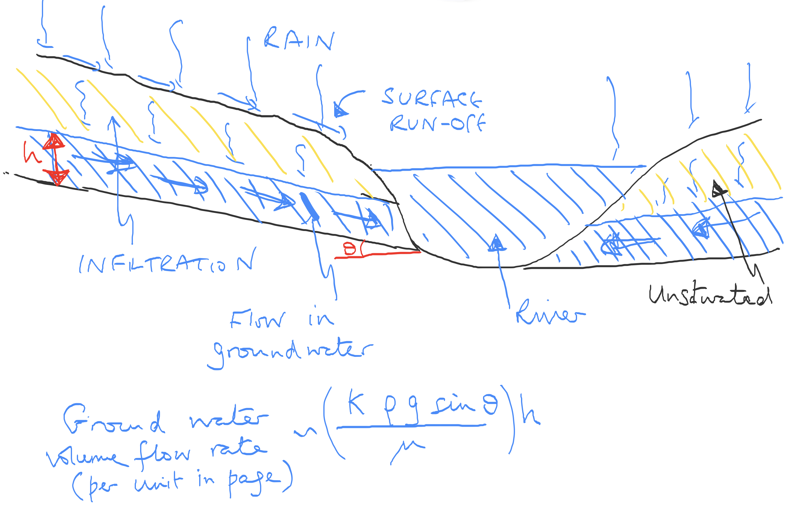
Fig. 4.29 The processes of a groundwater flood.

The flow running below ground typically has a velocity which depends on the permeability of the formation (e.g. soil) and the slope of the catchment. The flow may then drain into the base of a river. Analogous models for the groundwater flow can be developed to predict the flow into the river (see Example Sheet 2).

In some cases with limestone formations, the water table may rise very quickly leading to outflow from the side of hills, and this can lead to rapid flooding downstream.