10.1. Wind Power

In this lecture we will outline some of the key environmental factors related to wind power generation and develop some simplified models to help us understand how these effects influence the development of wind farms.

There are four aspects we will focus on.

1. The location of the wind farm and the relation of this to the wind field.

2. The intermittency of the wind, in terms of turbulent fluctuations on a short time scale, diurnal fluctuations and seasonal fluctuations.

3. The detail of how the turbine extracts energy from the wind.

4. How the layout of an array of turbines means they interact with each other. Pulling this all together enables us to assess the potential power generation from a wind farm, and the temporal variability of this power. This is key to understand if we wish to provide a constant supply of electricity from a wind powered grid.

Location

First, the location of the wind farm and its relation to topography and other obstacles such a trees or buildings can have a major impact on the local wind field experienced by the turbines. These issues primarily impact onshore wind turbine arrays. To assess these effects, recall that the large scale wind is produced in the atmosphere by forcing on scales larger then hundreds of kilometers.

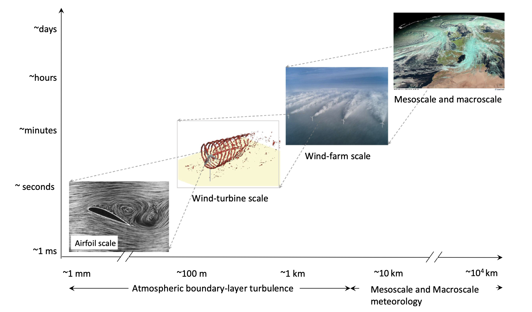
Fig. 10.1 The time and length scales of winds. From Porte-Agel et al. (2020).

As these winds flow over the land, the surface provides a frictional drag on the wind, leading to a reduction in the wind speed, and a region called a boundary layer develops above the ground, where the wind adjusts from the high values at altitude to much lower speeds at the surface. The structure of the boundary layer over flat land still depends on whether the surface is covered in trees or buildings, or is primarily open fields, and it may extend a few hundred metres above the surface as shown in Fig. 10.2.

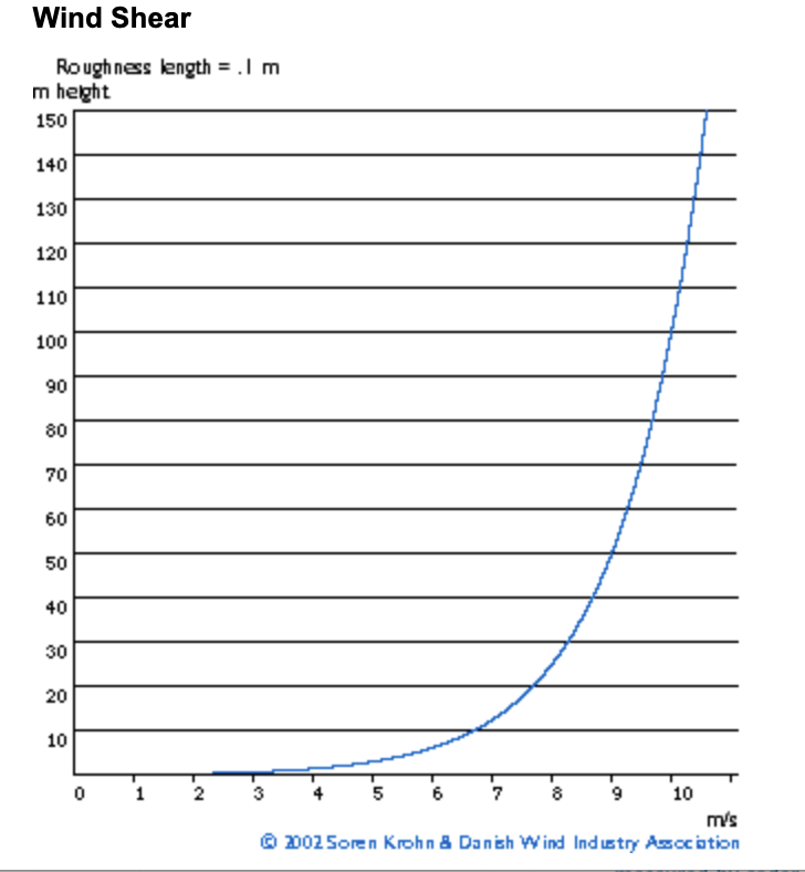
Fig. 10.2 Wind shear as a function of wind speed. From the Danish Wind Industry Association.

If there is an urban canopy or intermittent tree canopy, this adds more disturbance to the boundary layer, changing the velocity profile downwind. Also, there may be a shadow zone downwind where wind speeds are smaller.

Surface topography also has a major impact on the structure of the boundary layer, wind speeds on the windward side of the topographic feature are typically higher, and at the top of the hill the speed may be faster than elsewhere. However on the leeward side, there may be some separation of the wind, and recirculation, leading to reduced wind speeds. These effects can extend considerable distances downwind of the topography.

There can also be strong thermal effects related to mountain-valley topography, with katabatic winds composed of cold dense air being channelled downslopes in the evening as the mountain cools and cold air then sinks down into the valley. In contrast, as the mountain warms up in the day, the air rises, and draws air up from the valley. These winds have a strong diurnal component and although local may have a major impact on the wind field, and hence the power generated by a wind turbine.

Finally, near the land-sea interface, there are typically sea-breezes driven by cold air displacing warmer air, with these being onshore in the morning as the land warms up more rapidly, and offshore in the evening as the land cools down more rapidly. Some wind farms are located near shore to take advantage of this effect, rather than relying on the prevailing winds.

Intermittency

The second key factor related to calculating wind turbine performance relates to the intermittency of the wind. Typically, the wind field has high frequency turbulent fluctuations with periods of order 1-10 seconds, such as you may experience with gusts of wind. However, the wind field also has fluctuations from day to night (diurnal variations), especially with katabatic wind effects and onshore/offshore wind fields. Third, the background regional wind intensity tends to be very seasonal, with higher winds in the winter in general, but there are fluctuations in the wind intensity on periods of a week to a few weeks, related to the passage of weather patterns of high and low pressure, which are on a continental scale.

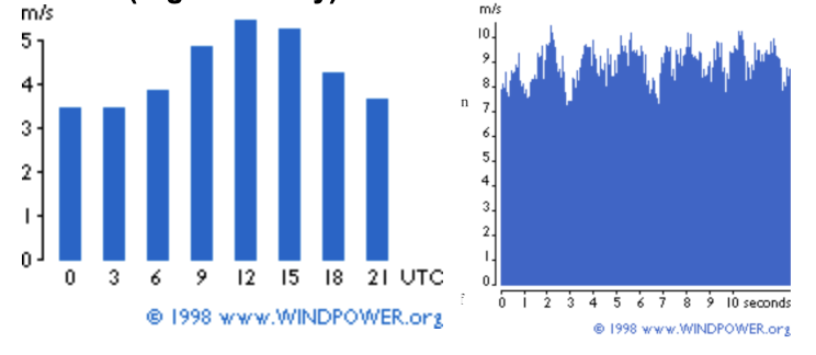
Fig. 10.3 The variability of wind speed at different time scales. Left, variation of the course of a day. Right, variation over the course of a few seconds. From the Danish Wind Industry Association.

For example Fig. 10.4 shows data from the UK wind power production in February 2023 shows periods of weeks when there is significant wind power generation and then weeks when there is less wind power generation.

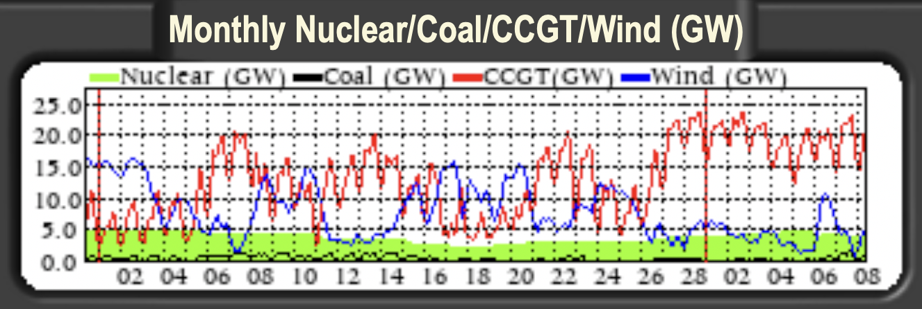
Fig. 10.4 UK grid power production over the course of February 2023 by source.

In addition to the fluctuations in the wind owing to the passage of weather systems and seasonal variations, there is also a more general variation in the wind speed from day to day and hour to hour.

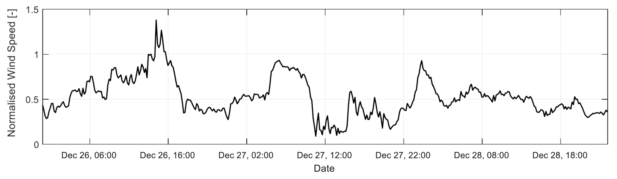
Fig. 10.5 day to day and hour to hour associated with the variations in the strength of the wind

If a record of wind speeds is collected then, with sufficient samples, the wind speed follows a so-called Weibull probability distribution, which can be written in the form of three parameters \(\beta\), \(\eta\) and \(\gamma\):

\[f(T) = \frac{\beta}{\eta} \left( \frac{T - \gamma}{\eta} \right)^{\beta - 1} e^{-\left( \frac{T - \gamma}{\eta} \right)^{\beta}}\]

This distribution has a long tail of high wind speeds of the form shown in Fig. 10.6.

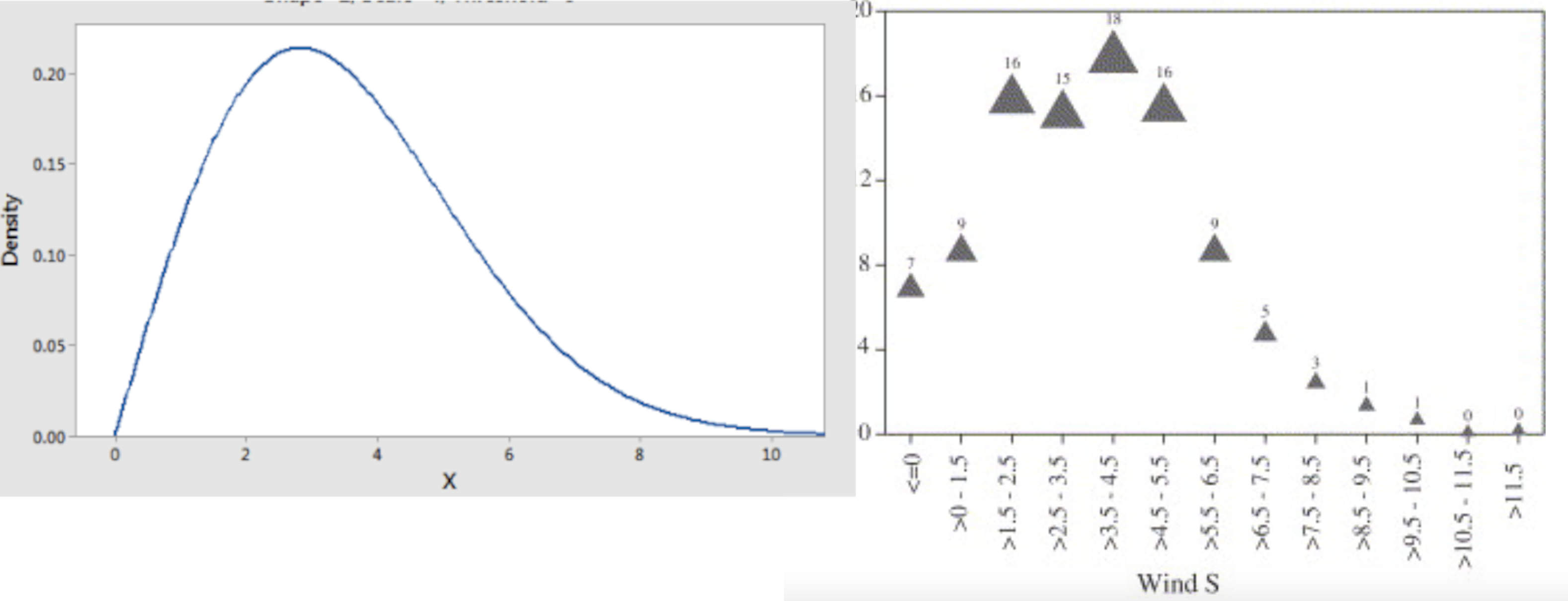
Fig. 10.6 An example Weibull distribution (left) and wind speed data (right).

In assessing the power a turbine can extract from the wind over time, we need to establish the statistical distribution of the wind speed, and then combine this with the power produced by the turbine for a given wind speed to derive the average power produced. Since the wind speed is variable, a turbine with a given maximum power will only produce a fraction of that power on average, as there will be days where the wind speed is too slow to generate that peak power.

A second impication of this wind data is that there is considerable intermittency on a range of different time scales. This means that in order for a purely renewable energy generation system using wind turbines to produce a continuous supply of power, some storage of energy is needed. Furthermore, this storage should be comparable to the total power used over a period of several weeks. We will come back to storage solutions in a later lecture.

Power generated by a turbine

The next problem to address is the power produced by a turbine as a function of wind speed, now we have a description of the wind speed distribution. In practice this is a complex problem to solve, as it depends on the turbulent flow or air through the turbine, including the turbulent fluctuations in the wind as well as the mean wind. Many modern wind turbines are so large that the span of the blades is of order 100 m and so they extend well into the atmospheric boundary layer. This means that the top of the turbine experiences a different wind speed than the lower parts of the blade, so the forcing on the blades is not independent of their position.

Nonetheless, it is useful to develop an expression for the power generated from a wind turbine for an idealised, uniform wind as a reference. Even this problem is rather difficult. However, all is not lost, and we can follow the approach of Betz to calculate a maximum value for the power generated. Having an estimate of the maximum theoretical power is useful as a reference for measured values of power generated in a real turbine, since it allows us to see if there is any scope for improvement in the design.

In developing our estimate, the physical idea we are exploring is that as the wind passes through the turbine it slows down and transfers some of its kinetic energy to rotational energy of the turbine rotors. In turn, these generate electricity through a generator. As a very simple back of the envelope estimate, you might say that if the wind speed is \(u\), and the turbine area \(A_T\), then the kinetic energy of the wind passing through the turbine is the product of the mass flux and the kinetic energy per unit mass

\[$E_k$ = (r A_T u) \frac{u^2}{2}\]

where \(r\) is the density of air. However, we can develop a better (but not perfect) estimate for the power production as follows. We assume that the wind has speed \(u\) upstream, which corresponds to the prevailing wind speed. As the wind approaches the turbine and drives the blades round, the air speed decreases to value \(v\) say at the turbine and on leaving the turbine and moving downstream, the wind slows down to further speed \(w\).

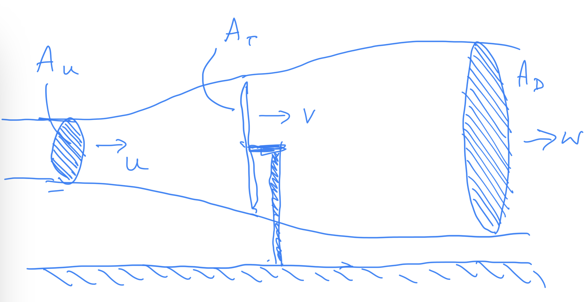
Fig. 10.7 A schematic of wind speed through a turbine.

We can use mass conservation to relate the air flow which passes through the turbine, \(Q\), say in terms of (i) the flow upstream of the turbine, which passes through an area \(A_u\) with (ii) that passing through the turbine, of area \(A_T\), and (iii) that downwind, when the flow has adjusted to speed \(w\), through an area \(A_D\), as shown in Fig. 10.7. This allows us to equate these quantities through conservation of mass

(10.1)\[Q = r A_u u = r A_T v = r A_D w\]

The force acting on the wind at the turbine, \(F\), drives the rotor arms. By conservation of momentum, this force equals the change in momentum of the flow from the upstream to downstream, giving

(10.2)\[Q u - Q w = F\]

Finally, the work done by the wind in driving the rotor is given by \(Fv\), and this matches the change in the energy of the air flow from upstream to downstream, so that

(10.3)\[Q \frac{u^2}{2} - Q \frac{w^2}{2} = Fv\]

In these equations, we know the value of \(u\), the upstream wind, and the area of the turbine \(A_T\). Thus, we want to try to combine the equations to find a relation between the power generated by the turbine, \(Fv\), and the values of \(u\) and \(A_T\). However, we do not have enough relations to do this exactly, but we can combine the expressions to express \(Fv\) in terms of \(u\), \(A_T\) and \(w\), the speed downstream, as follows

Equation (10.3) can be written

(10.4)\[Q (u - w) (u + w) = 2 Fv\]

Equation (10.2) can be written

(10.5)\[Q (u - w) = F\]

Replacing the term \(Q(u-w)\) in (10.4) with \(F\) (using (10.5)) we find

(10.6)\[u + w = 2 v\]

so the speed through the turbine is the average of the upstream and downstream air speeds.

Now we can use (6) to write the mass flow rate of air through the turbine as

(10.7)\[Q = r A_T \frac{(u + w)}{2}\]

Combining this with (10.4) we have the expression for the power generated

(10.8)\[Fv = r a_t U^3 (1 + l)^2 \frac{(1 - l)}{2}\]

where \(l = w/u\) is the ratio of the speed downwind to the speed upwind, and we know that \(0< l < 1\).

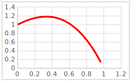
Fig. 10.8 Plot of \((1 + l)^2 (1-l)\) as a function of \(l\)

Although we do not know the value of \(w/u\), we can find the maximum value of \(Fv\) as a function of \(l\), and this will provide an upper bound on the power which can be generated. By differentiating the right hand side of (10.8) with respect to \(l\) we find that the maximum occurs when \(l = 1/3\), which means that the maximum power would be generated if the downwind speed has value \(u/3\). In this case, we find that the power has value

(10.9)\[Fv = 16 / 27 [r A_T u^3 / 2]\]

Comparing to the back of the envelope number above, we see that since 16/27 ~0.59, the turbine can extract less than 60% of the kinetic energy of the upstream wind passing through an area equal to that of the turbine rotors. In practice, this downwind speed is determined by the flow and does not equal \(u/3\), so the power is less than this maximum value. Typical turbines may have a range of values which could be as large as 30-40% at some wind speeds.

It is interesting to note that the power is proportional to \(u^3\), so that if the wind speed halves, the power produced falls to 1/8. This illustrates the crucial role of turbine placement in maximising the performance of a turbine; if the turbine is in shadow of an obstacle, with lower speeds than upstream, then the can power drop off dramatically. Also, the mean power generated by the turbine over a certain period depends on the number of days there is strong wind compared to weak wind, and even if a turbine is rated to produce a certain power, there may be many calm days when it produces a much more modest output.

To estimate the mean power which can be generated from a turbine, we can combine the probability distribution of the wind speed with a turbine power curve. The turbine power curve typically has an S shape (see Fig. 10.9), with the power increasing with wind speed according to the simple model above.

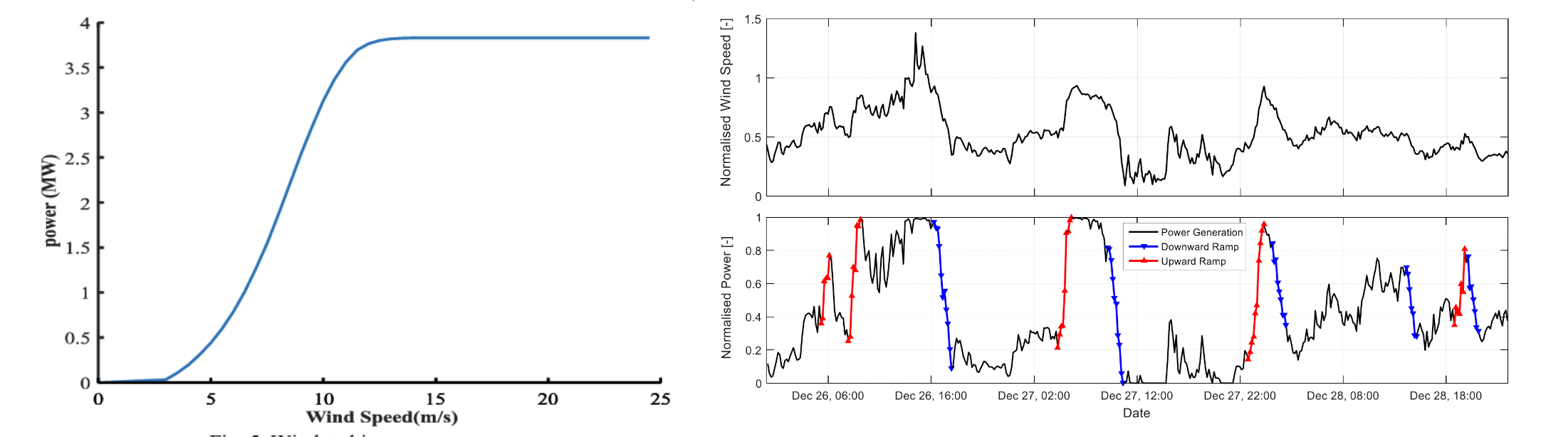
Fig. 10.9 Wind speed and power output.

Wind turbine power curve. Turbine cuts out at low speed and saturates at high speed. Illustration of the turbine power for given wind speed showing the amplification of changes in wind speed on the power production. However, at high winds, the turbine rotors tend to be rotated to prevent damage and the power output will be capped. Suppose (i) at a given location, the probability that the wind speed has value \(w\) is \(P(w)\), and (ii) the power generated by the turbine at wind speed \(w\) is \(F(w)w\), then the average power generated by this turbine at this site will be given by the expression

\[F = \int_0^{w_{max}} P(w) F(w) w dw\]

In general \(F\) is about 20-25% of the maximum power rating of a turbine given the distribution of the wind, and so on average a turbine only produces about 1/5-1/4 of the maximum rated power generation. This means that to generate 1 unit of power, 4-5 turbines with 1 unit of power as their maximum power generation capacity need to be installed.

Wake and array designs

Many wind turbines are installed in arrays, and the relative position of the turbines in such an array is crucial for the effective operation of the downwind turbines so that the air flow is not diminished from an upstream turbine.

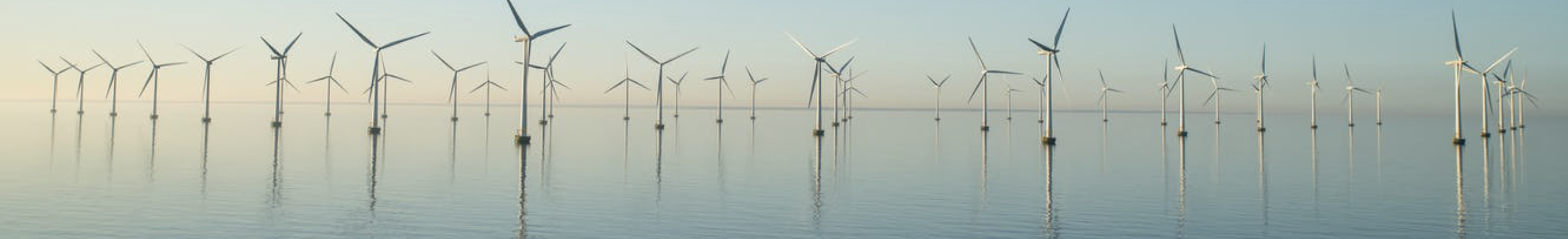
Fig. 10.10 An array of wind turbines.

We focussed on the power extraction in the previous section, and found that the air flow downwind has a reduced speed compared to the upwind region. This wake represents a momentum deficit in the air flow, and as the flow continues to move downstream, turbulent mixing between the wake and the surrounding wind flow leads to a gradual recovery of the momentum in the wake.

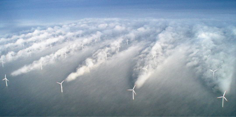
Fig. 10.11 A light fog reveals the wake effect behind turbines at Vattenfall’s Horns Rev wind farm off Denmark. Photo: Vattenfall.

Idealised model for the decay of momentum in the wake (Jensen Model)

Wake grows linearly downstream

\[r(x) = r(0) + l x\]

Speed adjusts to wind according to idealised model

\[U(x) = U_e - (U_e - U(0)) \frac{r(0)^2}{(r(0) + l x)^2}\]

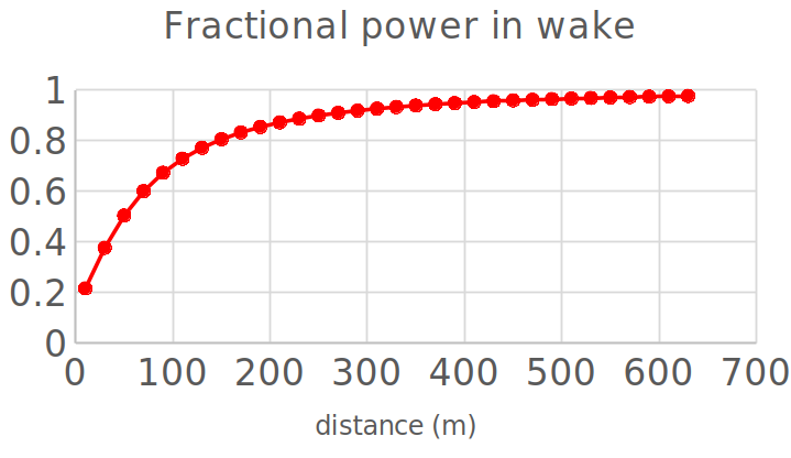
Fig. 10.12 The impact of wake on turbine power.

Placement of turbines downwind is crucial to avoid reducing power generation potential but also to maximise number of turbines on a given site. Wind direction can also impact the efficiency of turbines as seen in the image below showing data on the reduction in power generation downwind.