2.1. Groundwater Systems#
Water Demand#
The UK has a high demand per-capita for water, on the order of \(200 \ \mathrm{l}\) per day, per person. Of this, about 33% is used for toilets, and another 33% is showers, dishwashers and drinking (the bit that needs to be potable). Certain parts of the UK are under severe water stress.
But in addition to turning on the tap and using water for our regular ‘domestic’ life, many of the everyday products that we use all the time have a large water footprint. A water footprint refers to the total amount of water that it takes to make something. You can see the water footprint of some common foods in Fig. 2.1, and in the lecture we will go through in detail the water footprint to make one cup of coffee.
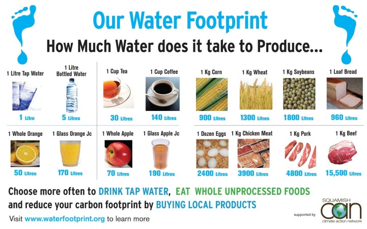
Fig. 2.1 The water footprint of various sundry goods. Image based on The water needed for the Dutch to drink coffee by Chapagain and Hoekstra (2003).#
Groundwater#
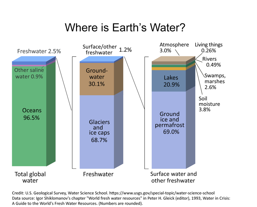
Fig. 2.2 The distribution of water on earth. Left, all water. Middle, fresh water. Right, surface water.#
Roughly 30% of Earth’s fresh water is in groundwater (Fig. 2.2), with most of the rest tied up in glaciers. How does water get into the ground? If we consider the mass balance of the hydrological cycle. Rain falls down on the ground, and approximately 30% of it returns to the atmosphere via evaporation, 30% returns to the atmosphere via transpiration, and 30% runs off the land through streams and rivers (which you’ll learn more about in Lectures 13-18). The balance of these processes will clearly differ all over the planet depending on vegetation cover, temperature, climate, and soil type (among many other things). But approximately ~10% seeps into the ground through a process called infiltration, or percolation (Fig. 2.3). This infiltration supplies water to the point beneath the surface where the pore space (the space between the grains of soil or rock) is full of water, or saturated, this is often called the water table. This process of infiltration of rainwater into groundwater is broadly termed recharge. Recharge is simply, precipitation minus runoff and evapotranspiration.
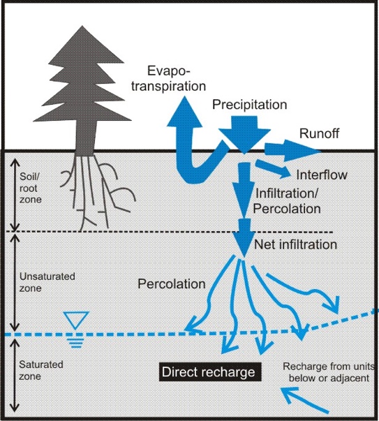
Fig. 2.3 A schematic showing the fluxes of water within, into and out of the groundwater system.#
Within groundwater systems, recharge brings water in, and discharge refers to where water is leaking out of the groundwater system. This can be into a body of water (stream, river, lake), or into the ocean (called submarine groundwater discharge), or directly onto land (groundwater sapping). What drives groundwater to flow from recharge to discharge, and how it may evolve along this flow path, will be discussed over the course of today and the next three lectures.
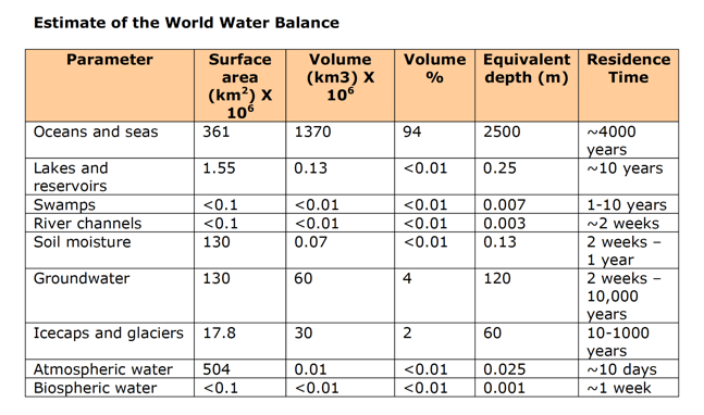
Residence Times#
Similar to Lecture 3, we can consider a groundwater system as a reservoir (or box) and think about the supply of water to that box as the recharge and the removal of water from that box as the discharge and ask ourselves what is the residence time of water in groundwater (Fig. 2.4)? What we find is that the residence time is very long (although a very large range!). There is a small flux in terms of recharge and discharge, and a large volume, and the calculated residence time is thousands of years!
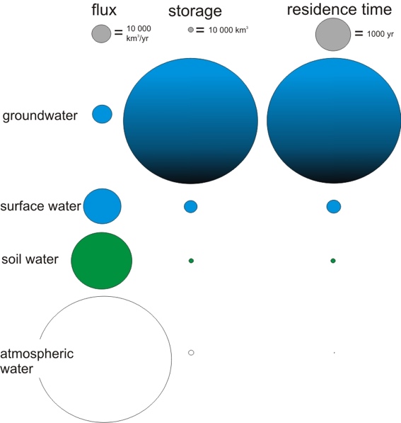
Fig. 2.4 The flux, capacity, and residence times for various water reservoirs on earth.#
We can verify this by measuring, or dating, the chemistry of groundwater. When groundwater was last in contact with the atmosphere, for example it acquires a certain chemical signature, that can decay as it flows through the ground. Some examples of these were given in the lecture. It was through this chemical dating of groundwater that some scientists in Canada discovered that some groundwater has been buried and isolated from the atmosphere for billions of years, and that there is a vast amount of deep salty groundwater below the fresh surface groundwater that we are interested in for drinking, agriculture and all the other things for which we need water.
This table, which was not in the lecture, gives a nice overview of where water is all over the surface and approximately how much time it spends in any one of those reservoirs.
Aquifers#
As we consider groundwater systems, we can first think about the key vocabulary we use to describe them (we did this above with infiltration, and runoff, and water table). Aquifer comes from two Latin words for water (aqua) and bear (ferre) – and literally means water-bearing formation. It is the part of the ground below the water table where groundwater can not only exist, but there is enough space between the solid bits for groundwater to move. This is in contrast to an aquitard, which restricts (or retards – slows) water flow, and at the extreme and aquiclude stops (or precludes) water flow all together.
Within aquifers we talk about confined aquifers and unconfined aquifers. Some schematics of these are in in Fig. 2.5, and were shown in the lecture. A confined aquifer has an aquitard (or aquiclude) which stops or slows (confines) the water in the groundwater system. An unconfined aquifer has the ground surface as the upper bound.
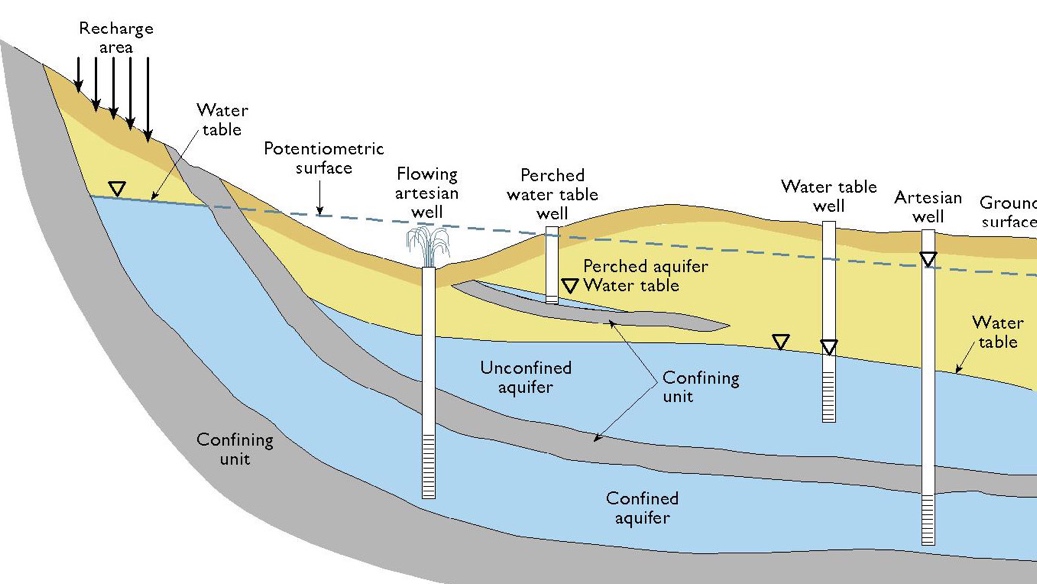
Fig. 2.5 Schematic figure showing the anatomy of different kinds of aquifer.#
In the schematic in Fig. 2.5, ‘confining units’ are aquitards, and the unconfined and confined aquifers are labelled. It should be clear that the residence time of water in a confined aquifer is much longer than it is in an unconfined aquifer. Furthermore, if we think about a toxic chemical spill at the surface, an unconfined aquifer will get more of the toxin leaking into it as it isn’t protected, where a confined aquifer often is protected from surface chemicals through the aquitard, or confining unit.
Sometimes – even often - the pressure in a confined aquifer is greater than that at the surface. This is in part because of gas in the water that exsolves, and chemical reactions that take place and generate gas. The gas can’t escape because of the confining units, therefore, when a well is drilled into the high-pressure aquifer, the water moves from high pressure (depth) to low pressure (surface). This is called an artisan well.
Porosity#
In general the water storage ability in an aquifer is controlled by the porosity. Porosity is the space between the grains of sand or particles of rock where water can exist. We measure porosity by assessing the total volume of sediment and then the total volume of voids. This is done assuming a density of the material.
There are four things that control the porosity of a system where groundwater moves
Grain shape and packing
Grain-size distribution
Degree of compaction
Degree of cementation
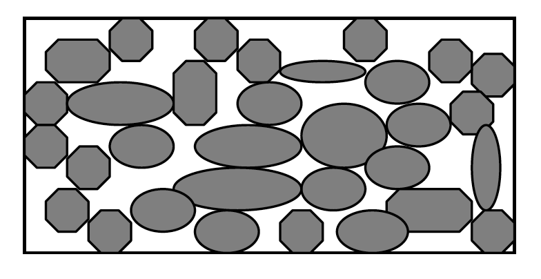
Fig. 2.6 A cartoon showing how porosity is controlled by grain geometry.#
In general, porosity ranges from 10 to 60% in most places where groundwater might be found. Perfectly uniform spheres with cubic packing have a porosity of ~48%. Most materials are less than that, you can get bigger than that if there are fractures or large void spaces in the rock.
We can think about the groundwater system more broadly in a similar way to how we did in the last lecture for the carbon cycle. This reiterates the importance of mass balance. The inputs of water to the system come from precipitation (\(P\)) as well as groundwater that moves laterally in from another part of the region (\(G_{in}\) more on this in the next lecture!). The outputs are from evapotranspiration (\(E_{tp}\)), runoff (\(R\)) on the surface, and runoff through the ground (\(G_{out}\)). If we consider the amount that is stored in the groundwater for a particular area (\(S\)), we get a mass balance equation similar to that used for the carbon cycle in the previous lecture.
Of these things, really only \(P\) and \(R\) can be measured (precipitation and runoff). The others we need to use a model to estimate. Always remember that we often assume steady state, which means that the amount in the groundwater (\(S\)) is not changing with time. We can consider if this is a reasonable assumption! Therefore