3.3. The extent of sea ice

The formation of sea ice plays an important role in both the radiative balance in the polar oceans as well as the polar component of large-scale oceanic circulation.

Radiation model for sea ice formation

Let’s consider a reasonably complete picture of the various heat fluxes which determine the growth of sea ice in the polar oceans, and then we’ll return to a very simplified model to understand the essential dynamics.

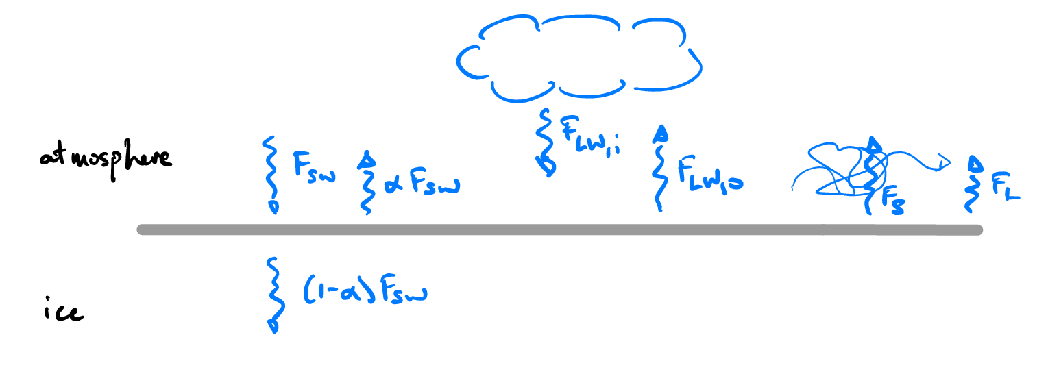
Fig. 3.11 Simplified radiation model for the growth of sea ice.

A simplified version of the complex balance of radiative forcing on sea ice is as follows.

1. The surface ice receives incident, short wavelength solar radiation \(F_{sw}\).

2. A fraction, \(\alpha\), of the incident short-wavelength radiation is reflected, where \(\alpha\) is the albedo.

3. A fraction, \((1-\alpha)\), of the incident short-wavelength radiation is transmitted into the ice below the surface, and subsequently into the ocean below.

4. If the atmosphere is at temperature \(T_A\) then the ice receives long wavelength radiation \(F_{LW,i} = \sigma T_A^4\) from the atmosphere and transmits outgoing radiation \(F_{LW,o} = \sigma T_s^4\), where \(T_s\) is the surface ice temperature. The difference between these fluxes thus gives a net outgoing heat flux

   (3.2)\[\begin{split}F_{LW} & = \sigma T_S^4 - \sigma T_A^4 \\ & \simeq 4\sigma T_s^3(T_s-T_A)\end{split}\]

   where the approximation follows because \(T_s \simeq T_A\) (at least when measured in Kelvin).

   It’s perhaps worth recalling that the power radiated from a body (ice or atmosphere) at a given temperature \(T\) is given by the Stefan-Bolztmann law

   (3.3)\[F = \sigma T^4\]

   where \(\sigma = 5.67\times10^{-8}\ \mathrm{W~m^{-2}~K^{-4}}\).

5. The ice looses sensible heat through a surface flux, which is mostly forced by convection in the air, \(F_s = h_T (T_s - T_A)\). Here \(h_T\) is a heat transfer coefficient which might, in general, depend on the wind strength, but for simplicity here is taken as a constant.

6. Finally, the ice looses energy in the form of a latent heat flux associated with sublimation (evaporation) of the ice into the atmosphere,

   (3.4)\[F_L = h_s(T_s - T_A)\]

   where \(h_s\) is a heat transfer coefficient for sublimation / evaporation which incorporates the latent heat of phase change.

Formation of ice on the ocean surface

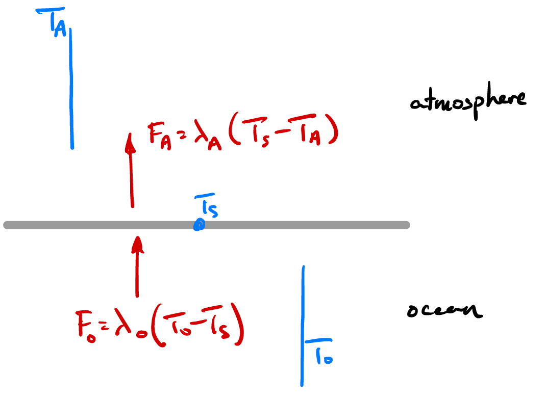
Fig. 3.12 Conditions for the formation of the first ice, when the surface temperature of the ocean \(T_s = T_m\).

Ice forms in the polar oceans during the polar winter when the atmospheric temperature becomes significantly below zero. Prior to ice formation, the condition at the ocean surface is that the heat flux from the ocean must equal the heat flux to the atmosphere, the balance of which determines the surface temperature. Hence

(3.5)\[\begin{split}F_o & = F_A \\ \implies \lambda_o(T_o-T_s) & = & \lambda_A(T_s-T_A)\end{split}\]

which we can re-arrange to give the surface temperature

(3.6)\[T_s = \frac{\lambda_o T_o+ \lambda_A T_A}{\lambda_o + \lambda_A}\]

Ice begins to form when the surface temperature goes below the melting / freezing temperature \(T_s < T_m\), so that

(3.7)\[T_A < T_m - \frac{\lambda_o}{\lambda_A}(T_o-T_m) < T_m\]

Growth of sea ice

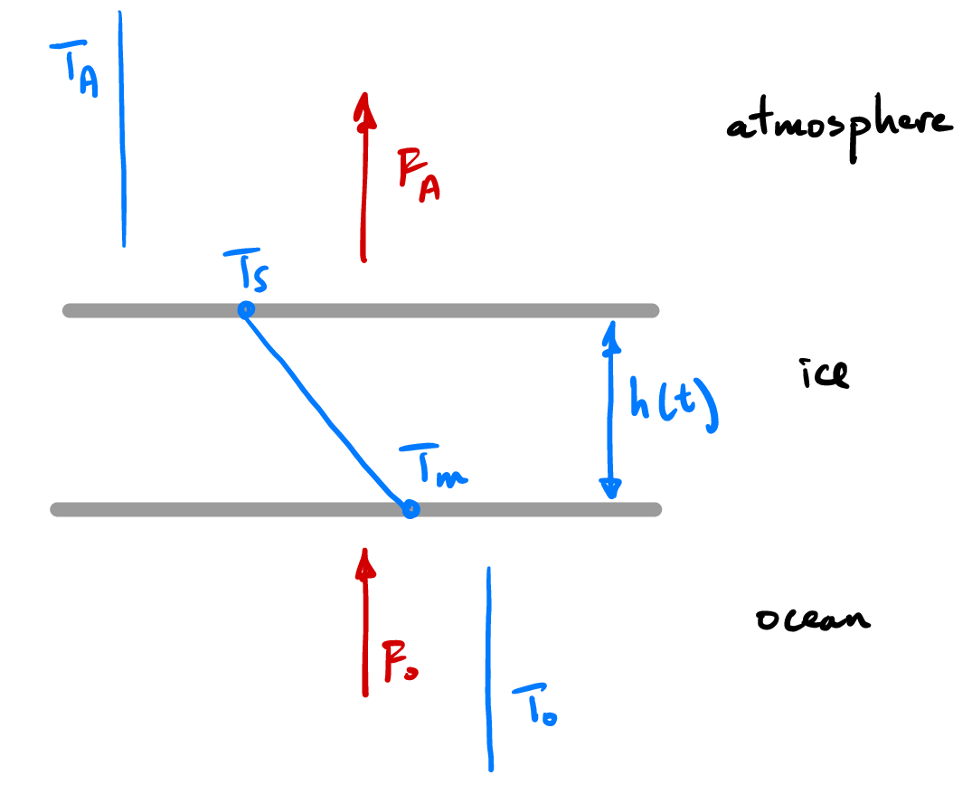
Fig. 3.13 Simple thermal model for the growth of sea ice.

Once the ice is growing, we assume that the ice grows in a quasi-steady manner, and hence that there is a linear thermal profile through the ice. The growth of ice is driven by the heat flux to the atmosphere, \(F_A\), which balances the diffusive flux of heat across the ice,

(3.8)\[F_A = \lambda_A(T_s-T_A) = k\frac{T_m-T_s}{h}\]

and we can then infer (from equation (3.8)) that the surface temperature is given by

(3.9)\[T_s = \frac{T_m + (\lambda_A h/k)T_A}{1+\lambda_A h/k}\]

If we consider a fixed ocean temperature, and hence a fixed oceanic heat flux \(F_o = \lambda_o(T_o-T_m)\), and recalledd that the growth of ice is limited by the release of latent heat on solidification and any heat flux from the ocean, we can construct the equation governing the growth of ice:

(3.10)\[\rho L \dv{h}{t} = k\frac{T_m-T_s}{h} - F_o\]

So already we can see that the surface temperature approaches the freezing point for thin ice, \(T_s \to T_m\) as \(h\to0\), while for thick ice it approaches the atmospheric temperature \(T_s \to T_a\) as \(h\to\infty\). We can also see that, from (3.9), \(T_s \simeq T_A\) once \(h \ge k/\lambda_A\).

The equation governing the growth of ice (equation (3.10)) can be now be re-written as

(3.11)\[\rho L \dv{h}{t} = \frac{\lambda_A(T_m-T_A)}{1+\lambda_A h/k} - F_o\]

which is now an (admittedly awkward) ODE in thickness \(h\) alone (otherwise it is known temperatures and material parameters). Interestingly, we can observe the following behaviour. At early times when \(\lambda_A h/k \ll 1\) the ice growth is approximately constant \(h \sim t\), whereas at intermediate times \(\lambda_A h/k \gg 1\) the ice grows as the square-root of time \(h \sim \sqrt{t}\). Finally at late times the oceanic heat flux balances the surface cooling so that the ice reaches a steady state thickness,

(3.12)\[h(t \to \infty) = \frac{k}{\lambda_A}\left[\frac{\lambda_A(T_m-T_A)}{F_o} - 1\right]\]

Note that for ice \(k \simeq 2\ \mathrm{W~m^{-2}~K^{-1}}\) and \(\lambda_A \simeq 20\ \mathrm{W~m^{-2}~K^{-1}}\) the length scale \(k/\lambda_A \simeq 10\ \mbox{cm}\) and the final steady state thickness is a few metres.

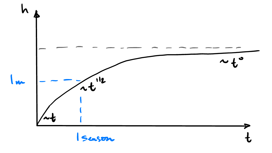
Fig. 3.14 Ice thickness over time using a radiative balance at the ice surface.

Melting of sea ice

The melting of sea ice can occur from two directions. The ocean temperature may be warmer, indicating a higher oceanic heat flux leading to thinning from the base of the ice. Correspondingly, and often intuitively given the surface seasonal radiative balance, the atmospheric temperature may increase above the melting temperature. Both an increase in surface sensible air temperature and oceanic heat flux are relevant for the response of sea ice thickness to climate change.

Since we have considered a fixed ocean heat flux in our solidification examples (above) let’s focus on the case of a high air temperature \(T_A > T_m\). In this case, the surface temperature is at the melting temperature \(T_s = T_m\) and, since it is still in contact with the liquid water ocean, so is the base of the ice. After an initial transient the ice is therefore uniformly at the melting temperature, and the melt rate is simply given by

(3.13)\[\rho L \dv{h}{t} = F_A - F_o\]

recalling of course that \(F_A = \lambda_A(T_m - T_A) < 0\) since now \(T_A > T_m\). Hence, the ice melts from both the top and bottom.

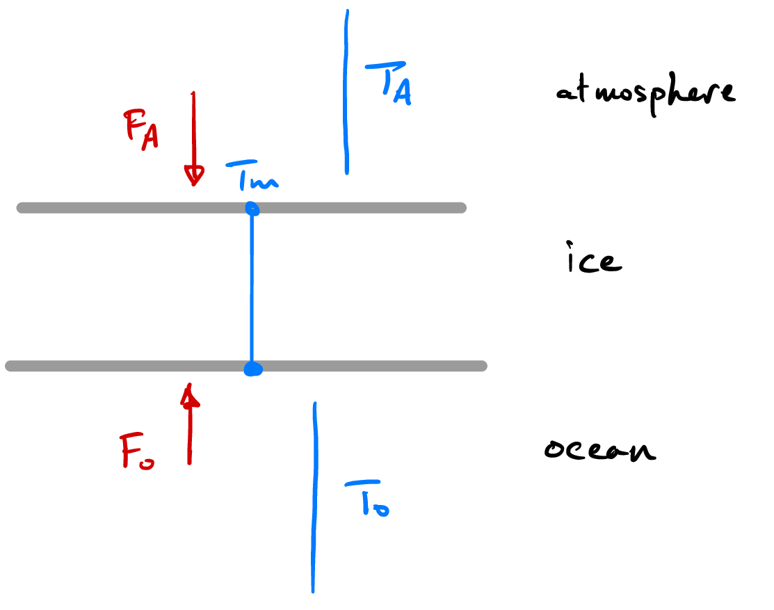
Fig. 3.15 Schematic temperature structure in melting ice.

Seasonal cycle

Putting all of these pieces together we can begin to understand the seasonal cycle of sea ice. As the summer radiation wanes, the surface temperature follows the atmospheric temperature with some lag. Then, as the air temperature plummets the surface temperature finally crosses the freezing point and ice begins to form. This ice layer grows and thickens, but more slowly as it thickens, and effectively insulates the ocean beneath which always has a surface temperature \(T_m\). Finally, as the air temperature warms the ice becomes isothermal at the melting temperature and melts (from the top and the bottom). The discontinuous jump in surface temperature occurs when the ice disappears, at which point the surface is no longer pinned to the freezing temperature. The seasonal cycle is sketched schematically in Fig. 3.16.

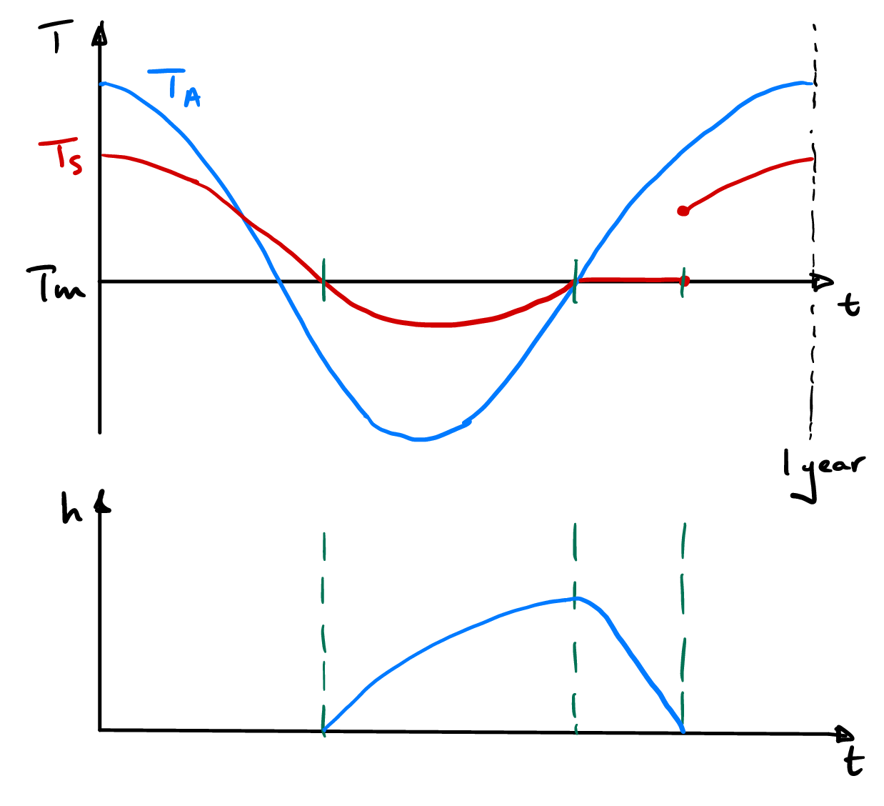
Fig. 3.16 Schematic seasonal cycle of ice surface temperature \(T_s\) and ice thickness \(h\).

It is worth also mentioning that, while we have concentrated on the thermodynamic growth and melting of sea ice, the thickness distribution of sea ice is a function of both the thermodynamic growth (which accounts for the thin end of the thickness distribution) and advection of ice resulting in ridging and rafting (which accounts for the long, thick tail of the ice thickness distribution). A representative ice thickness distribution is given in Fig. 3.17.

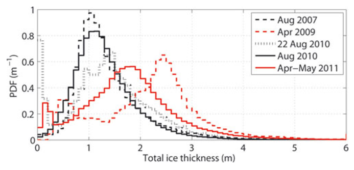
Fig. 3.17 Ice thickness distribution in the Arctic ocean, from Renner et al. Annals. Glac. (2013).

Freezing salty ocean water

A significant aspect of the solidification of sea ice in polar waters is that ocean water is salty, not fresh. This means that ocean waters, with a salt concentration of approximately \(C_o \simeq 0\ \mathrm{wt\%}\), freeze at a temperature \(T_L \simeq -1.8^\circ\mathrm{C}\). The result is fresh water ice (salt does not get incorporated in the ice lattice) and more salty and cold surface waters.

This thermodynamics of freezing salty ocean water is therefore determined by a binary eutectic phase diagram. This plots the phase behaviour as a function of temperature \(T\) and the concentration \(C\) of the dominant salt, NaCl (here in weight percent) as shown in Fig. 3.18. On the phase diagram the liquidus line, \(T_L(C)\) distinguishes the concentration-dependent freezing temperature. Below the liquidius nearly pure solid ice crystals form, bathed in a cold and salty interstitial brine. As temperatures fall below the eutectic temperature \(T_E\) both solid ice and salt crystals form.

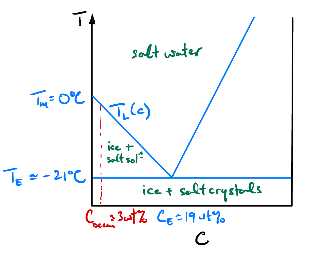
Fig. 3.18 Phase diagram of sea ice as a function of temperature \(T\) and concentration \(C\ (\mathrm{wt\%})\). Note theliquidus line \(T_L(C)\) which marks the concentration-dependent freezing point, and the eutectic temperature and concentration, \(T_E,\ C_E\), which is the temperature below which both ice and salt crystals form.

The impact of the salt on the solidification of sea ice is important both locally and globally. Locally, the solidification of ice from brine results in a porous block of ice, which has important implications for the thermal and mechanical properties of the ice. But on a global scale, it is the rejection of salt on freezing which produces very cold, salty and therefore dense waters in the polar regions that has major implications for the dynamics of the global overturning circulation.