4.2. 1D model of drainage into a river

In a catchment there are a series of drainage zones, each flowing into a stream and then into the river, in a hierarchical way. This leads to the question of how to build a model for the whole drainage basin which is more complex that the idealised bucket model. We also may use such a detailed model to assess the value of \(\lambda\) in the model based on the more detailed physical processes in a more complete model. To this end we consider the next step of development of the model which is to consider the drainage along the land from the watershed to a stream as shown in Fig. 4.10.

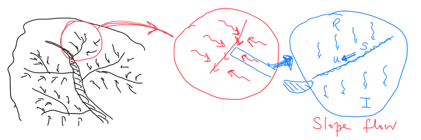
Fig. 4.10 A more detailed surface drainage model showing the fractal nature of drainage networks.

Flow speed

Extending our model from 0D into 1D, adding a spatial dependence, we are going to need to assess the dominant controls on the fluid dynamics. The speed of the flow down the slope may be given in terms of the permeable flow relation; D’Arcy’s law, which we discussed in Section 2.2. Flow through crops, wooded land or other surfaces provide the effective porous media with an effective permeability, \(k\).

In this case, the flow speed will be of the form

Units!

\[\begin{split} u &= \mathrm{m~s^{-1}} \\ \rho &= \mathrm{kg~m^{-3}} \\ g &= \mathrm{m~s^{-2}} \\ \theta &= \mathrm{radians} \\ \mu &= \mathrm{kg~m^{-1}~s^{-1}} \\ k &= \mathrm{m^2} \\ \end{split}\]

(4.5)\[u = \rho g \sin{(\theta)} \frac{k}{\mu}\]

over the surface. The effective permeability may be quite high near the ground.

Deriving the advection equation

We now wish to derive a relation describing how water is stored on and moves down our slope. We will do this by considering the flow of water into and out of a small space element on our slope, \(\delta x\), as shown in Fig. 4.11.

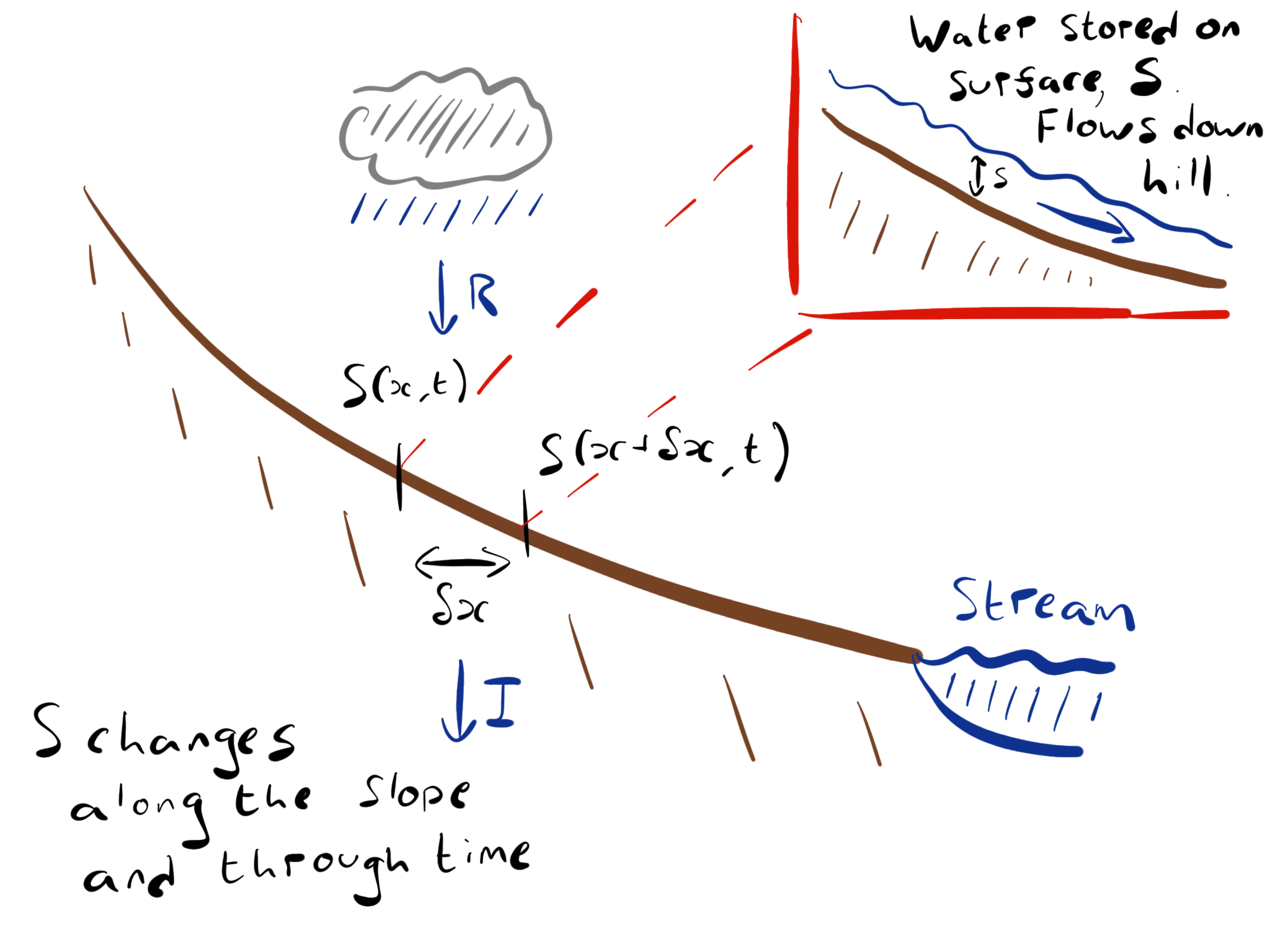
Fig. 4.11 A schematic model showing how surface water, \(S\), flows downhill towards a stream.

The total amount of water stored in our space element is denoted by \(S\). The sources of water to our element will be flow in from up slope, and rain, \(R\). The sinks of water from our element will be flow out of the element down slope, and infiltration into the ground, \(I\).

The flow, \(Q(x,t)\), at a point is calculated as the product of the amount of water \(S\), multiplied by its speed \(u\). Given that our speed down the slope, \(u\), is constant in this formulation, we can use our diagram in Fig. 4.11 to identify the flow in from up-slope as \(u S(x,t)\) and the flow out down-slope as \(-u S(x+\delta x, t)\).

Therefore, balancing all inputs and outputs of water to our space element over a short period of time, \(\delta t\), we get the relation:

Units!

\[\begin{split} Q &= \mathrm{m^3~s^{-1}} \\ R, I &= \mathrm{m~s^{-1}} \\ S &= \mathrm{m^2 \ (m^3 m^{-1})} \\ L &= \mathrm{m} \\ \end{split}\]

\[(S(x, t + \delta t) - S(x, t)) \delta x = R \delta x \delta t - I \delta x \delta t - (u S(x + \delta x, t) - u S(x, t)) \delta t\]

And so dividing through by \(\delta x\) and \(\delta t\), and then taking the limit in which \(\delta x\) and \(\delta t\) go to zero gives us the differential equation

(4.6)\[\frac{\partial S}{\partial t} = R - I - u \frac{\partial S}{\partial x}\]

This is called the advection equation and it governs the change of surface storage along the surface from the watershed to the stream (in the direction of the flow along the surface).

Solving the advection equation

To find the flux of water into the river, we need to evaluate \(S(x,t)\) at the river edge (i.e \(x=L\)). Therefore we need to solve the advection in case. Given that the advection equation has a characteristic speed \(u\), we expect solutions that encode this. In order to use this intuition, we can apply a coordinate transform that moves us into the frame of reference of a parcel of water moving down the slope at a speed \(u\).

Units!

\[\begin{split} W &= \mathrm{m^2} \\ \eta &= \mathrm{m} \\ \tau &= \mathrm{s} \\ \end{split}\]

\[S(x,t) = W(\eta, \tau)\]

Where \(\eta = x - u t\) and \(\tau = t\).

This leads to the relations:

\[\begin{split}\begin{align} \frac{\partial W}{\partial t} &= - u \frac{\partial W}{\partial \eta} + \frac{\partial W}{\partial \tau} \\ \frac{\partial W}{\partial x} &= \frac{\partial W}{\partial \eta} \end{align}\end{split}\]

Derivation

We want to derive the new derivative relations for our coordinate transformation, Therefore, writing out the total derivative in \(W\):

\[\dd{W} = \pdv{W}{\tau} \dd{\tau} + \pdv{W}{\eta} \dd{\eta}\]

We can then “divide through by \(\dd{t}\)”, which while not rigorous, is fine for a physical system like this one

\[\pdv{W}{t} = \pdv{W}{\tau} \pdv{\tau}{t} + \pdv{W}{\eta} \pdv{\eta}{t}\]

Then evaluating the derivatives of our coordinate transform

\[\pdv{\tau}{t} = 1 \quad \pdv{\eta}{t}=-u\]

and then substituting into our previous equation gives the required result

\[\pdv{W}{t} = \pdv{W}{\tau} - u \pdv{W}{\eta}\]

We could then repeat this analysis to get the equivalent result for \(\pdv{W}{x}\).

Substituting these relations into (4.6) we get

\[\frac{\partial W}{\partial \tau} = R - I\]

We can solve this equation by integrating with respect to \(\tau\) (recalling \(R\) and \(I\) are constant). This gives us a solution for a given (i.e. constant) value of \(\eta\).

\[W(\eta, \tau) = W(\eta, 0) + (R - I) \tau\]

Where \(W(\eta, 0)\) is our constant of integration representing the initial condition. This allows us to construct a characteristic diagram for the system, showing solutions in the \(x\) - \(t\) plane, along lines of constant \(\eta\). This is shown in Fig. 4.12.

We want the solution when \(x = L\) (i.e. the value of \(S\) at the stream), shown as the dashed line intersecting the \(x\) axis in Fig. 4.12.

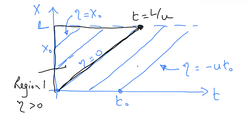
Fig. 4.12 The characteristic diagram for the advection equation, showing lines of \(\eta = \mathrm{constant}\) on the \(x\) - \(t\) plane.

There are two regions for the solution:

• Region 1. The set of points where \(x = L\) and \(t \lt \frac{L}{u}\), for which lines \(\eta = \mathrm{constant}\) start on the x-axis at time = 0 (e.g. the line starting at \(x_0\)). For each of these lines, the time at which they reach the distance \(x = L\) is \(t = \frac{(L-x_0)}{u}\); i.e. the time for the line of constant \(\eta\) starting at \(x=x_0\) at \(t=0\) to reach the line \(x = L\). Therefore the value of \(W\) (and hence \(S\)) at time \(t\) and at \(x = L\) is \(W=(R-I)t\).

• Region 2. The other region corresponds to the points \(x=L\) and \(t \gt \frac{L}{u}\). In this region the lines of constant \(\eta\) which reach \(x = L\) for \(t \gt \frac{L}{u}\) start at \(x = 0\) at a time \(t_0 \gt 0\). Hence, the time to reach the line \(x = L\) is \(\frac{L}{u}\), and so at \(x = L\), \(W = (R-I) \frac{L}{u}\) for \(t \gt \frac{L}{u}\).

As a result, the flux at \(x = L\) is given by

\[\begin{split}\begin{align} u S &= u (R - I) t && \mathrm{for} && t \lt \frac{L}{u}\\ u S &= (R - I) L && \mathrm{for} && t \geq \frac{L}{u} \end{align}\end{split}\]

Matching this latter solution for equilibrium with the equilibrium solution for the bucket model, we can identify the parameter \(\lambda\) in the bucket model as

\[\lambda = \frac{L}{u}\]

This is the time constant for reaching equilibrium between the surface water accumulation and flow into the streams.