2.3. How we measure and understand water movement#
A concept that derives from the idea of a distribution of hydraulic head is the distribution of a piezometric or potentiometric surface across a groundwater catchment. This is the level to which the water table would rise (or fall) if it were not confined in the subsurface (Fig. 2.15). In an unconfined aquifer, this is just the water table – or where the water is found. In the case of a confined aquifer, we can think of this having a water table that represents the total potential energy within the confined aquifer. More intuitively, if we were to drill a well into the aquifer, the water level would rise to this level (which differs from the actual water table itself). This is called the potentiometric surface (or piezometric surface) and is given by the red dashed line below. Sometimes this is above the actual surface and indicates that if you drilled a well into that aquifer, the water level would come up above the surface.
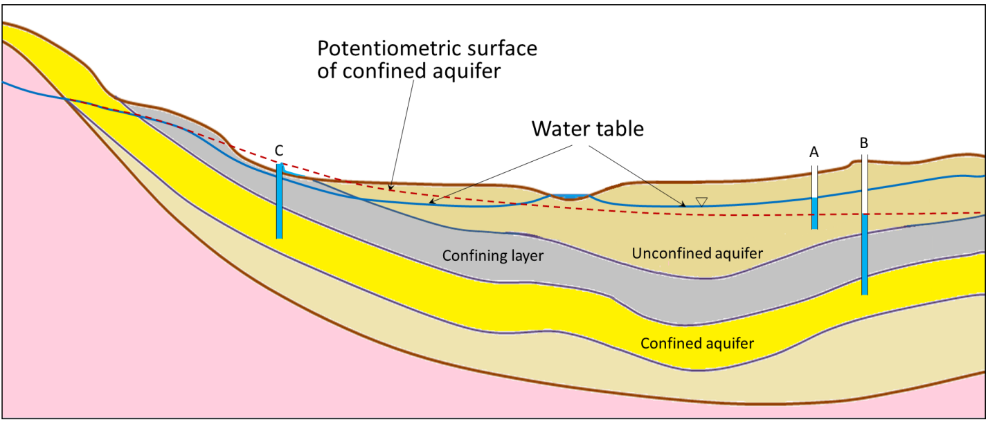
Fig. 2.15 The structure of an aquifer and the potentiometric surface. Notice how differences between the water table and potentiometric surface relate to sub-surface structure.#
We can think of lines of equal pressure in a groundwater system, which are known as equipotential lines, and use this to draw flow lines, which will flow perpendicular to the pressure lines. This allows us to create a map like Fig. 2.16 showing where and how groundwater will move. What is clear from this sort of a figure is that groundwater doesn’t always move in a straight line. We can do a simple calculation for the amount of time it would take groundwater to move 100 meters from a recharge area to a discharge area (e.g. a stream) but in reality, we can see the flow lines/paths aren’t linear. Furthermore, to calculate things like the flow velocity in a groundwater system, we need to know aspects of the system like the permeability or hydraulic conductivity very well. How are these things determined?
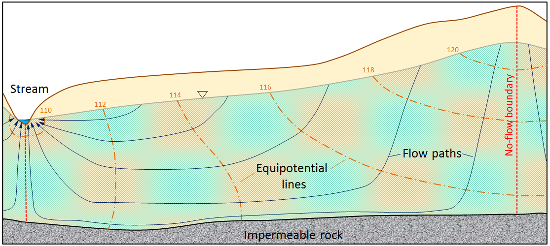
Fig. 2.16 The structure of an aquifer and the potentiometric surface. Notice how differences between the water table and potentiometric surface relate to sub-surface structure.#
One way that we can determine the hydraulic conductivity and other key properties of a groundwater system is to perform a pumping test (Fig. 2.17). During a pumping test we remove water from one well and monitor the drawdown of water from a second well that is some (known) distance from the first well.
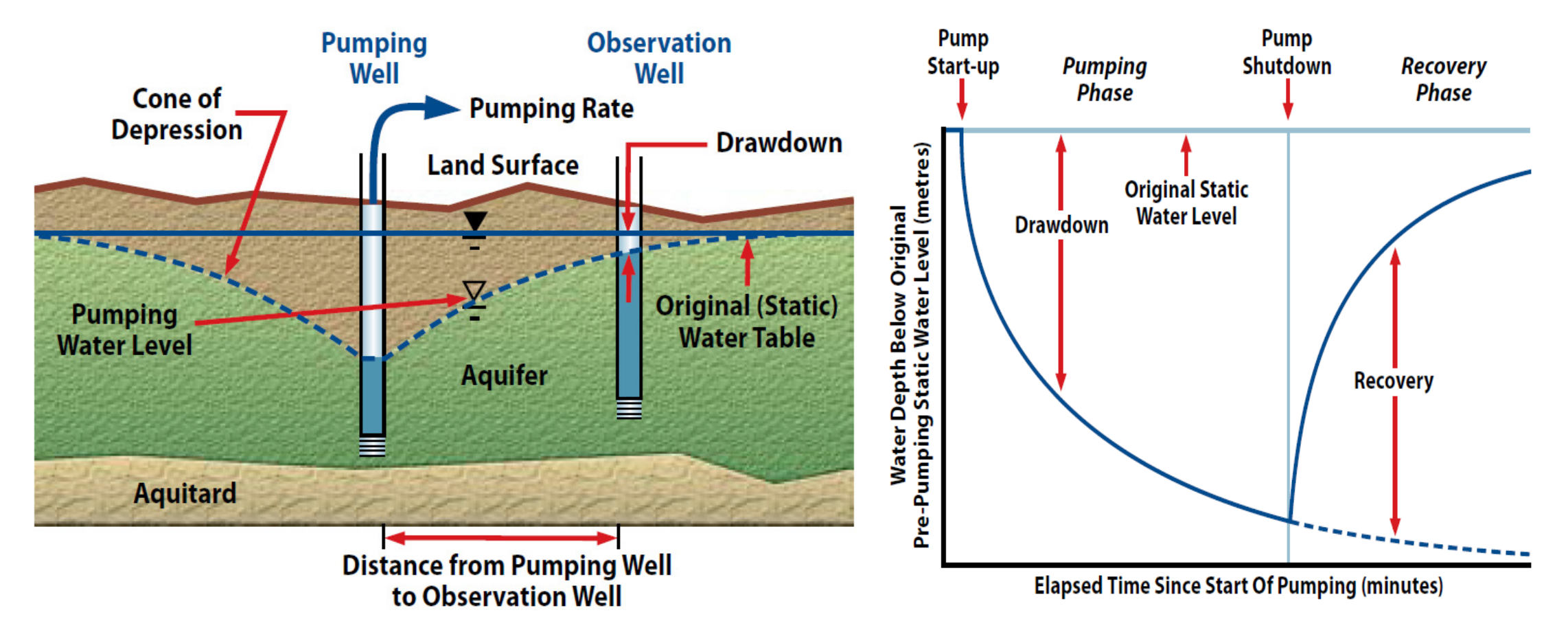
Fig. 2.17 A schematic of a pumping test for an unconfined aquifer (left) and an idealised drawdown curve for this test (right). Images from here.#
Let’s consider this idealised case where we are performing a pumping test in an aquifer. We can define several geometric parameters associated with our pumping test. For example, our flow rate will be \(Q\), the thickness/height of our aquifer is \(b\), and the height of water is \(h\). A schematic of this is shown below in Fig. 2.18.
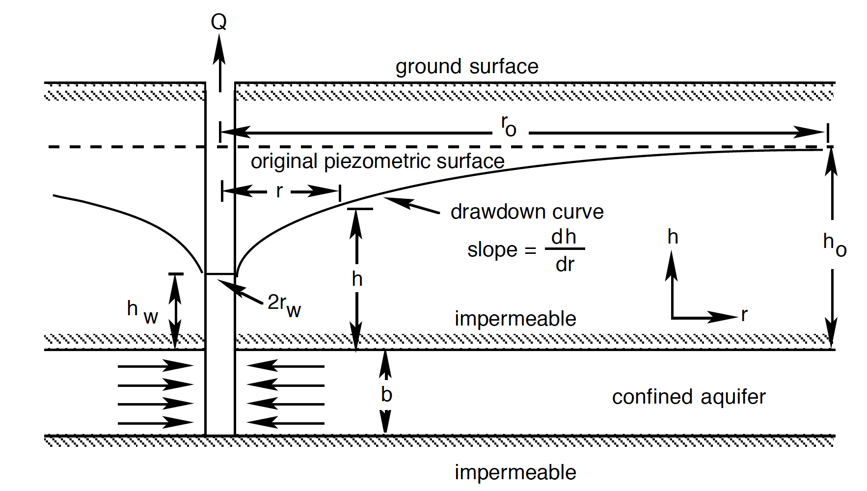
Fig. 2.18 The geometry of an idealised confined aquifer in a pumping test.#
In an idealised sense, the drawdown will be conical in shape, and we can think about the evolution of that cone (with time) in terms of the change in the radius versus the change in the height to the side of the cone \(\left( \dv{r}{h} \right)\). This is the slope of the piezometric surface at radius \(r\) from the centre of the pumping well. A schematic of this is given in Fig. 2.19. The drawdown of the piezometric (or potentiometric surface) results from the reduction of pressure in the aquifer due to pumping).
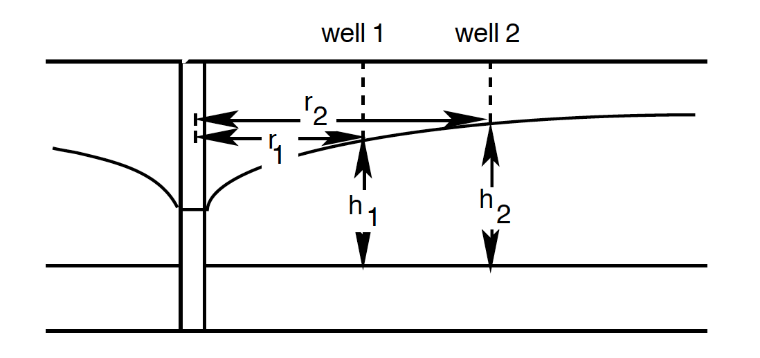
Fig. 2.19 The change with radius down the borehole follows a piezometric surface .#
To continue this calculation we have to make a few assumptions:
The aquifer is homogenous and isotropic (the same in all directions)
The well penetrates the whole of the confined aquifer, so the flow is horizontal
We will keep \(Q\) constant (the flow is steady). This keeps other things (like the size of the cone) constant as well.
If we consider a cylinder of the aquifer of radius \(r\), and height \(b\) around the well, then if we apply Darcy’s Law, the rate of flow out of the well (and into the well from the groundwater) – \(Q\) – is given by
Where \(A\) is \(2 \pi rb\). This means all together:
We can then separate our variables:
And integrate both sides from \(h_w\) to \(h_o\) and \(r_w\) to \(r_o\):
But because \(\frac{Q}{2 \pi b K}\) is constant, we can bring that out of the integral:
Which can be solved to give:
Which we can rearrange to make something called the Thiem equation:
Here \(h_o\) is the height from the aquifer to the surface before any pumping and \(r_o\) is the radius before any pumping, so \(h_w\) and \(r\) just track the evolution of the height and radius of the cone as the pumping test evolves. It follows that if \(Q\) is fixed, and \(b\) and \(K\) don’t change, there should be a linear relationship between \(h\) and \(\ln{r}\).
In most cases we are using a certain pumping rate (\(Q\)) and then measuring the response of the cone, and we want to understand the hydraulic conductivity of the system (or the permeability). We can rearrange Eq. (2.14) to solve for permeability:
One of the major assumptions in a test like this is that we are at steady state, and the cone shape and size isn’t changing with time (adding in a time dependence would change the maths quite a bit). This isn’t strictly true as the longer we pump a groundwater system, the more the cone will widen and deepen. However, at some point you do reach a point where the rate of change is really very small over time, and we can assume a ‘quasi’ steady state (Fig. 2.20).
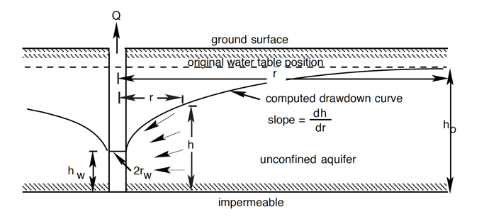
Fig. 2.20 The geometry of an idealised unconfined aquifer in a pumping test.#
We can think of lots of ways this will be different if the geometry of the subsurface means our assumptions don’t hold. But it is also different when there are very different hydraulic conductivities involved (Fig. 2.21)!
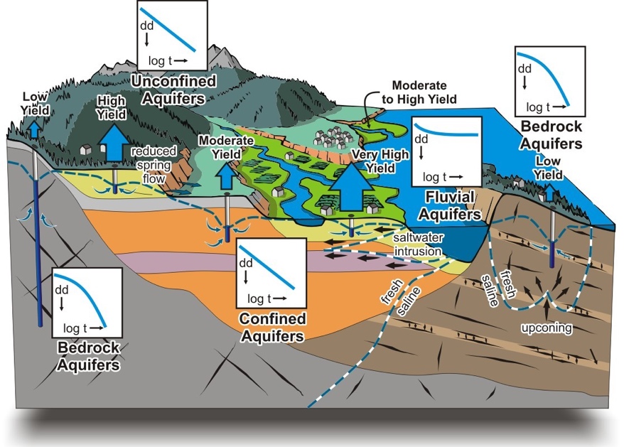
Fig. 2.21 Hydraulic conductivity can vary a lot with geology!#