5.3. The chemistry of pollutants#
Oxidation, phase-transitions, steady-state burdens
The chemistry of pollutants: we will review the mechanism of loss of pollutants in the atmosphere. This occurs there four main routes: gas-phase oxidation, heterogeneous uptake, photolysis and gas-to-aerosol partitioning. We will calculate how these different processes impact the lifetime of a pollutant and calculate the steady state burden of \(\mathrm{NO_2}\).
Aims:
To describe the rates of changes of pollutants in the atmosphere through different processes.
To calculate the steady state burden of a pollutant in the atmosphere.
To calculate how the steady state will change under different conditions.
Key points:
Constituents in the atmosphere can undergo (pseudo)first order decay and second order decay.
Photolysis is an example of first order decay that is important for photolabile molecules like \(\mathrm{NO_2}\).
The steady state of represents the concentration of a species when its rates of production and loss are balanced.
Chemical kinetics allows us to predict how the steady state will change.
Rates of change in the atmosphere#
If we have a chemical species, \(\mathrm{A}\), that is lost via a process in the atmosphere, we can plot the change in its concentration as a function of time as shown in Figure 5.12:
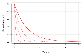
Fig. 5.12 Rate of change of the concentration of a species \(\mathrm{A}\) for varying values of the rate constant \(k\)#
We can represent the loss of \(\mathrm{A}\) in this situation as:
The greater the magnitude of \(k\), the “faster” the loss of \(\mathrm{A}\).
Rather than just observing how \(\mathrm{A}\) will change we can solve the equation above to calculate \(\mathrm{[A]}_t\).
Given that \(k\) is a constant we can then write:
and therefore
We can use this graph and the equations above to define the time constant, \(\tau\), as the time taken for the concentration of \(\mathrm{A}\) to be reduced by a factor of \(\frac{1}{e}\).
The smaller this time constant the greater the loss of \(\mathrm{A}\) with time and hence the shorter its lifetime.
The example above holds for the case where \(\mathrm{[A]_t}\) is independent of factors other than \(k\). This occurs through many processes but not all.
Consider the slightly more complex reaction:
On first glance we expect this to be a second order process (first order in \(\mathrm{A}\) and first order in \(\mathrm{B}\) so second order overall). However, if the concentration of \(\mathrm{[B]}\) doesn’t change much over time (for example because \(\mathrm{B}\) is present in large excess) then we can make the approximation that \(\dv{\mathrm{[B]}}{t} \simeq 0\), which allows us to consider \(\mathrm{A}\) as undergoing pseudo-first order kinetics (\(\mathrm{[B] \sim}\) constant and so it can be folded into our second order rate constant, \(k_2\), to yield a pseudo-first order rate constant, \(k^\prime_2 = k_2 \mathrm{[B]}\)). The time constant for \(\mathrm{A}\) is now given by:
More complex again, what about a chain reaction:
where \(\mathrm{A}\) is our initial reactant, \(\mathrm{B}\) an intermediate product and \(\mathrm{C}\) the final product of the reaction. Following the same procedure as above we can write:
Solutions for these equations for \(k_1 = 1 \ \mathrm{s^{-1}}\) and \(k_2 = 2 \ \mathrm{s^{-1}}\) are shown below.
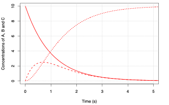
Fig. 5.13 Rate of change of the concentrations of species \(\mathrm{A}\) (solid line), \(\mathrm{B}\) (dashed line), and \(\mathrm{C}\) (dotted line), for \(k_2 = 1\).#
For the case where \(k_1 = 1 \ \mathrm{s^{-1}}\) and \(k_2 = 10 \ \mathrm{s^{-1}}\) we have:
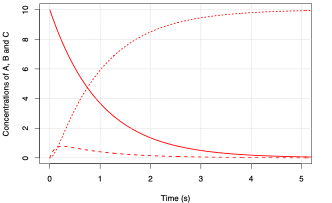
Fig. 5.14 Rate of change of the concentrations of species \(\mathrm{A}\) (solid line), \(\mathrm{B}\) (dashed line), and \(\mathrm{C}\) (dotted line), for \(k_2 = 10\).#
What you will notice from the figures above is that the intermediate \(\mathrm{B}\) is short-lived relative to \(\mathrm{C}\) and that as the value for \(k_2\) increases the peak concentration of \(\mathrm{B}\) decreases. The time it takes for B to reach an almost steady concentration is \(\sim \frac{1}{k_2}\). In the limit where \(k_2 \gg k_1\) we can make the approximation:
where the subscript \(\mathrm{ss}\) is used to note that we are considering the intermediate \(\mathrm{B}\) to be in steady state.
Following this through, we can re-write the remaining equations which describe our complex reaction (making the substitution \(\mathrm{[B]_{ss}} = \frac{k_1}{k_2} \mathrm{[A]}\)):
In doing so we have greatly reduced the complexity of this reaction system.
In the atmosphere there are many examples of compounds that can be considered to be in steady state.
Examples of first order decay#
Photolysis is a good example of first order decay.
Here the rate of change of our species (say \(\mathrm{NO_2}\)) is dependent on the photolysis coefficient.
This depends on the flux of photons from the sun, the absorption cross-section of \(\mathrm{NO_2}\) and its quantum yield.
The main challenge is to calculate \(J_\mathrm{NO_2}\) (see lecture_23).
The rate of a heterogeneous process is usually expressed in terms of the uptake coefficient, \(\gamma\), which is defined as the fraction of molecules colliding with the surface that are permanently lost from the gas phase.
According to the kinetic theory of gases, the rate of collision of a species \(\mathrm{A}\) at the surface, per unit area, is \(\mathrm{[A]} \frac{c}{4}\), where \(\mathrm{[A]}\) is the concentration (\(\mathrm{molecules \ cm^{-3}}\)) of species \(\mathrm{A}\) and \(c\) is the mean molecular speed of the gas molecules (\(= \sqrt{\frac{8RT}{\pi M}}\)).
The rate of removal of molecules at the surface can therefore be expressed as a first-order process with rate:
\(S\) is the surface area of the atmospheric particles (N.B. per unit volume of gas, often called the surface area density and has units of, for example, \(\mathrm{cm^2 \ cm^{-3}}\)). As well as providing data on the rate of removal of trace gases by aerosol particles, uptake coefficient measurements can be used to deduce the mechanisms of the heterogeneous processes.
Examples of pseudo-first order decay#
Many trace gases in the atmosphere are approximately constant in concentration with time. An example is the hydroxyl radical \(\mathrm{OH}\) whose concentration is roughly \(10^6 \ \mathrm{molecules \ cm^{-3}}\) during the day. \(\mathrm{OH}\) acts as the main detergent in the atmosphere reacting with almost all the other trace gases and pollutants that are emitted into the air. For example:
In this reaction the concentration of \(\mathrm{M}\) is unaffected but the concentration of \(\mathrm{OH}\) is reduced. However, there is a sufficiently large source of \(\mathrm{OH}\) such that it has no impact on the \(\mathrm{[OH]}\) so that we can write:
We can make use of this to predict the concentration of \(\mathrm{NO_2}\) (or \(\mathrm{HNO_3}\)):
where \(k = \mathrm{[OH][M]}\).
Steady state calculations#
In the example above we have implicitly made the assumption that \(\mathrm{[OH]}\) is in the steady state. Steady state was introduced in the chain reaction at the start of the lecture (and in 1A Chemical Kinetics). Steady state is an important approximation we often make use of in the atmosphere. Many pollutants are in steady state because their chemical loss processes are fast. How fast do they need to be? It depends on over what timescale we are interested in. As we saw in Section 5.2 \(\mathrm{[NO_2]}\) has changed a lot over the last 165 years. However, day to day we say that the \(\mathrm{[NO_2]}\) is fairly similar. During the COVID pandemic what caused the large decrease in \(\mathrm{[NO_2]}\) was a change in its emissions (source) rather than a change in its loss (sink).