5.1. An overview of the atmosphere#
Structure, composition and radiative processes
Aims:
To describe the basic structure of the atmosphere and understand what physical processes lead to the distinct “layers” present in Earth’s atmosphere
Recap on the radiative budget of the atmosphere and how different constituents affect the Earth’s radiative balance.
Outline the key radiatively important gases and particles present in the atmosphere.
Key Points:
The Earth surface is heated by incoming short-wave length radiation from the sun that is re-emitted out at longer wavelengths. This causes the lower layers of the atmosphere to decrease in Temperature as an air parcel ascends (a negative lapse rate \(\frac{dT}{dz}\)).
In the middle atmosphere, around \(30 \ \mathrm{km}\), ozone (\(\mathrm{O_3}\)) forms a layer (the ozone layer) which absorbs incoming short wave radiation and re-emits radiation at longer wavelengths leading to local heating.
This combination of a negative lapse rate in the troposphere and a positive lapse rate in the stratosphere means that air is well mixed in the troposphere but stratified in the stratosphere.
The gases and particles present in the atmosphere can absorb, scatter or re-emit radiation.
Molecules with a permanent dipole can absorb outgoing long-wave radiation and re-emit this, leading to the greenhouse effect.
Certain aerosols can scatter incoming shortwave radiation, cooling the surface.
\(\mathrm{CO_2}\), \(\mathrm{CH_4}\) and \(\mathrm{O_3}\) are key greenhouses gases that have changed in atmospheric abundance considerably due to anthropogenic activities
Introduction to the atmosphere#
We can consider the atmosphere divided into two main parts, dealing with the stratosphere (\(15-50 \ \mathrm{km}\)) and the troposphere (\(0\) to \(10-15 \mathrm{km}\)) as essentially separate regions with, in many respects, different photochemical and transport processes dominating. A very important first question is why this distinction can be made and why it is useful to do so. We should also ask why higher altitudes are not considered. The answers rest with the physical structure of the atmosphere – which is itself a function of both physical processes (gravity, buoyancy effects) and photochemistry and spectroscopy (absorption of visible solar radiation by \(\mathrm{O_2}\) and \(\mathrm{O_3}\), and emission in the infra-red by \(\mathrm{CO_2}\)). This leads to both a physical barrier between the two regions and quite different photochemical environments, these aspects are discussed below. We must start by looking at atmospheric vertical structure.
Variation of atmospheric pressure with altitude#
Depending on definition, the atmosphere can be taken to be a few 10s or perhaps \(\mathrm{100 \ km}\) thick. The gravitational constant can be taken to be \(g = \mathrm{9.81 \ m \ s^{-2}}\) throughout. The surface pressure of the atmosphere is thus determined by the total mass of atmosphere. The change in pressure \(\dd{p}\) following a displacement \(\dd{z}\) can be written as
where \(p\) is pressure, \(\rho\) is the ambient air density and \(z\) is altitude.
Since \(pV = nRT\), we can write \(\rho = \frac{Mn}{V} = \frac{Mp}{RT}\)
where \(M\) is the mean molar mass of air. Taking the atmospheric temperature to be constant (N.B. an approximation we will review later) we can write
or
which can be integrated to give
which is the hydrostatic relation, where \(H = \frac{RT}{Mg}\) is the scale height, \(T\), is the temperature, and \(M\), is the mean molar mass of dry air (\(28.8 \ \mathrm{g \ mol^{-1}}\)).
Typical values of \(H\) are given in Table 5.1:
\(T \ \mathrm{/ \ K}\) |
\(H \ \mathrm{/ \ km}\) |
|---|---|
200 |
5.88 |
240 |
7.06 |
280 |
8.24 |
The result is that to a good approximation pressure decays exponentially with height with a pressure scale height \(H\) in km.
A useful approximation is to take \(H = 7 \ \mathrm{km}\). Up to an altitude of approximately \(90 \ \mathrm{km}\), the bulk composition of the atmosphere essentially \(\mathrm{N_2:O_2} = 4:1\). At higher altitudes, diffusive separation can occur with light molecules such as \(\mathrm{H_2}\) capable of leaving the atmosphere altogether.
Using the hydrostatic relation we can calculate that approximately 90% of the atmosphere is below \(15 \ \mathrm{km}\), 99% below \(30 \ \mathrm{km}\), and 99.9% below \(45 \ \mathrm{km}\).
By considering only the troposphere and stratosphere, we are thus ignoring only 0.1% of the atmosphere (by mass), although for some scientific problems and for issues such as radio transmission, that 0.1% is critical!
Deviations from a uniform temperature profile#
The observed atmospheric temperature profile is far from uniform (see below). Ignoring for the moment the region above \(50 \ \mathrm{km}\), the main features are decreasing temperatures with altitude up to \(\sim 15 \ \mathrm{km}\), with increasing temperatures above. We will now consider why this occurs, and critically, why it is important.
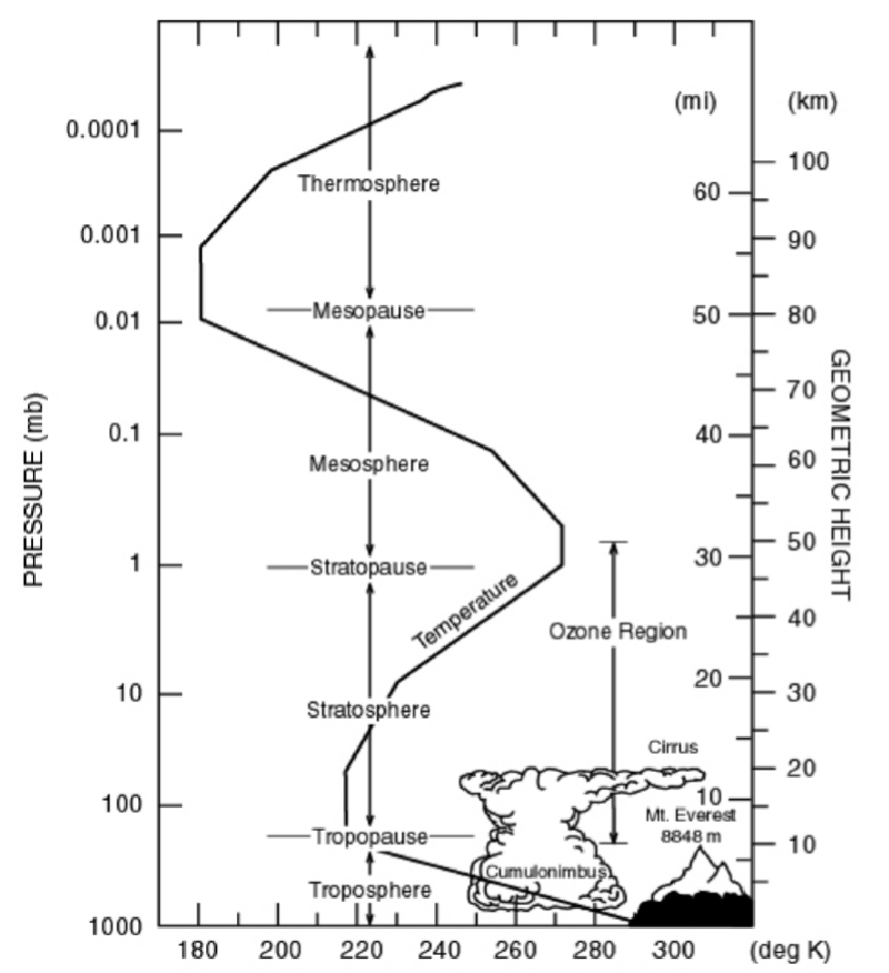
Fig. 5.1 Temperature structure of the atmosphere.#
The tropospheric temperature profile – heating from below#
The troposphere is heated largely from below - by solar radiation heating the Earth’s surface, heating the nearby air etc. The upshot is that this less dense air then has a tendency to rise (by processes equivalent to convection). As the air rises, it then encounters reduced pressures (see above) and therefore expands. In doing so it performs work on the external environment and if no external heat is applied, it must cool.
From the First Law of Thermodynamics: \(\dd{U} = \dd{q} + \dd{w}\)
where \(dU\) is the change in internal energy, \(dq\) the heat supplied to the system and \(dw\) the work done on it. If \(\dd{q} = 0\) (an adiabatic process i.e. no heat is given off to the environment) and \(\dd{w} = –p \dd{V}\) (expansion work, done by the rising gas), we can write
From the definition of enthalpy (\(H = U + pV\))
and substitution for \(\dd{U}\) gives
From the hydrostatic equation, the altitude dependence of pressure is given by
This allows us to write
where \(M\) (\(\mathrm{kg \ mol^{–1}}\)) is the molar mass. The definition of the molar heat capacity, \(C_p = \dv{H}{T}\) allows us to rewrite the above
So, the altitude dependence of temperature is given by \(\dv{T}{z} = – M g / Cp\)
Nitrogen and oxygen have very similar heat capacities of about \(29 \mathrm{J \ mol^{-1} \ K^{–1}}\) and so using an average molar mass for air of \(28.8 \mathrm{g} \ \mathrm{mol^{–1}}\), we get a rate of change of temperature with altitude
which is termed the (dry) adiabatic lapse rate, or \(\Gamma_{ad} = 9.8 \ \mathrm{K \ km^{–1}}\). In fact latent heat release from condensing water vapour heats the ascending air, leading to an average actual (environmental) lapse rate, \(\Gamma_{\mathrm{env}} = 6.5 \ \mathrm{K \ km^{–1}}\). This drop in temperature with altitude can be seen in Fig. 5.1
The stratospheric temperature profile – heating from above#
By contrast, the stratosphere is heated from above. Solar radiation is absorbed by \(\mathrm{O_3}\) (and at higher altitudes by \(\mathrm{O_2}\)).
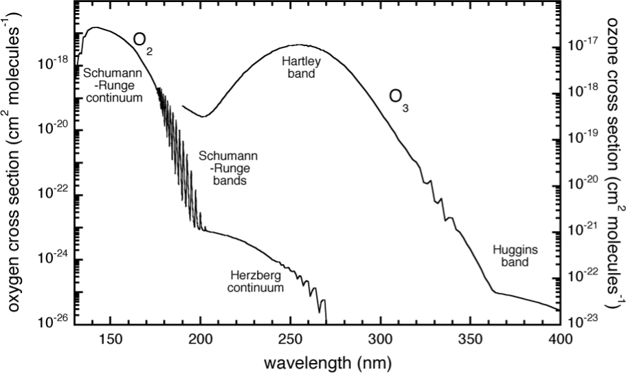
Fig. 5.2 Absorption bands of O2 and O3.#
Absorption of a photon of sufficient energy (\(h \nu\)) by \(\mathrm{O_3}\) in the Hartley and Huggins bands leads to the dissociation of \(\mathrm{O_3}\):
Recombination of \(\mathrm{O}\) in the presence of a third body, \(\mathrm{M}\), then releases the \(\mathrm{O - O_2}\) bond energy in the form of kinetic energy (heat)
What is a third body? Most likely \(\mathrm{N_2}\) as this is the most abundant gas in the atmosphere, but essentially \(\mathrm{M}\) could be anything.
Vertical stability of the atmosphere#
The atmospheric temperature profile is important because it determines the vertical stability (speed of vertical mixing) of the atmosphere.
Consider an idealised temperature profile (Fig. 5.3) with an environmental lapse rate (solid line) which in this illustrative case is taken to be larger (i.e. more negative) than the adiabatic lapse rate (dashed line). As a notional air parcel is displaced upwards from point A, it will cool at the adiabatic lapse rate by an amount \(\dd{T}\). However, at point B the environmental temperature is cooler by a further amount \(\dd{T}\).
The notional air parcel is thus warmer than its surroundings, is less dense, and will thus continue to rise – the air has become convectively unstable. Similarly, if the parcel is displaced downwards, the same argument leads to the parcel continuing to descend. In the troposphere where this condition is often satisfied, overturning readily occurs leading to rapid vertical transport and short transport times (typically weeks or less). If the environmental lapse rate \(\Gamma_{\mathrm{env}} \sim \Gamma_{ad}\), the air is said to be neutrally stable.
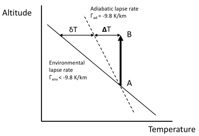
Fig. 5.3 Temperature profile for unstable conditions#
Consider the case when the vertical temperature gradient is positive (see Fig. 5.4). As above, upward displacement of the air parcel leads to a cooling of \(\Delta T\). However now the environmental temperature is higher by \(\dd{T}\), and so now the displaced parcel is cooler and thus more dense than its surroundings, and thus descends. As above, if it displaced downwards, it has a tendency to rise. Under these conditions the atmosphere is now stable to vertical displacements. These conditions are those found in the stratosphere, in which vertical transport is therefore slow (months – years).
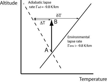
Fig. 5.4 Temperature profile for stable conditions#
The stable stratosphere thus acts as a ‘lid’ on the less stable troposphere, with the tropopause acting as a barrier to transport between the two regions. Gases emitted from the Earth’s surface thus become rapidly mixed throughout the troposphere, and are only transported slowly to the stratosphere. If they can be effectively scavenged when in the troposphere, they are unlikely to reach the upper atmosphere in significant concentrations.
Radiative properties of gases and particles#
In Section 1.2 we derived a simple energy balance model of the atmosphere. In this model we considered that the sun provides incoming short wave length radiation (\(\lambda < 500 \ \mathrm{nm}\)) and the Earth’s surface acts as a source of long-wavelength radiation. The difference in the emission of radiation from a black body can be described by Wien’s displacement law:
where \(\lambda_\mathrm{max}\) is the wavelength that is a the peak of the curve, \(b\) is Wein’s displacement constant, and \(T\) is the absolute temperature of the black-body in Kelvin.
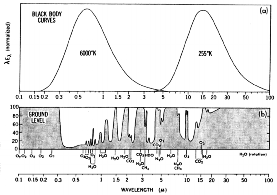
Fig. 5.5 Black body emission curves for the sun and Earth (a) and ground level emissivity (b).#
In panel (b) of Fig. 5.5 we can see that different molecules absorb the different wavelengths of radiation emitted by the sun and Earth. For an absorption to occur a molecule must be able to undergo a change in energy level (translational, rotation, vibrational or electronic). Absorption in the microwave region are typically associated with rotational transitions; Absorption in the infrared region typically are related to vibrational transitions; Absorption in the UV is typically associated with electronic transitions.
To absorb or emit radiation a molecule must possess a changing electric dipole. Molecules can have changing dipoles in several ways:
The molecule may have a permanent dipole – as the molecule rotates the dipole changes at the rotational frequency. For example:
\(\mathrm{O_2}\) or \(\mathrm{N_2}\): Both are homonuclear diatomic molecules. Neither have permanent dipole moments, hence neither have pure rotational absorption spectra.
\(\mathrm{CO_2}\): \(\mathrm{CO_2}\) is a linear symmetric molecule, and hence does not have a permanent dipole moment. As a result it does not have a pure rotational absorption spectrum.
\(\mathrm{H_2O}\): \(\mathrm{H_2O}\) is a bent symmetric molecule, and hence does have a permanent dipole moment. As a result it does have a pure rotational absorption spectrum.
The molecule may have a dipole which changes as the molecule vibrates:
\(\mathrm{O_2}\) or \(\mathrm{N_2}\): Both are homonuclear diatomic molecules. Because they have no dipoles, as they vibrate they can have no changing dipole – no vibrational spectrum.
\(\mathrm{CO_2}\): \(\mathrm{CO_2}\) does not have a permanent dipole moment, however as it vibrates, some of the vibrations create vibrating dipoles. As a result it does have a vibrational spectrum.
\(\mathrm{H_2O}\): As \(\mathrm{H_2O}\) vibrates, all of the vibrations create vibrating dipoles. As a result, like \(\mathrm{CO_2}\), it does have a vibrational spectrum.
These gases that can absorb the Earth’s outgoing long-wave radiation “trap” it and so distort the simple energy balance model we produced in Section 1.2.
The abundance of these gases has changed considerably over time.
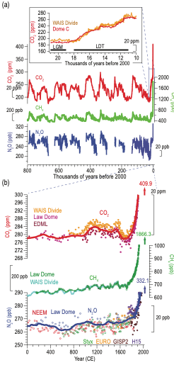
Fig. 5.6 Atmospheric well-mixed greenhouse gas (WMGHG) concentrations from ice cores. (a) Records during the last 800 kyr with the Last Glacial Maximum (LGM) to Holocene transition as inset. (b) Multiple high-resolution records over the CE. The horizontal black bars in panel (a) inset indicate LGM and Last Deglacial Termination (LDT) respectively. The red and blue lines in (b) are 100-year running averages for CO2 and N2O concentrations, respectively. The numbers with vertical arrows in (b) are instrumentally measured concentrations in 2019. Source IPCC AR6.#