10.5. Heating and Heat Transfer in Buildings#
Heat usage in buildings represents about 1/3 of the energy use in the UK, with domestic heating presently using natural gas as the dominant energy source. The transition in energy supply requires a change in the systems used for heating, and this opens up three opportunities:
Improved control of the heat supply.
Improved insulation to reduce the heat demand.
A change of system from gas boiler to heat pumps.
It is of interest to try to assess the relative potential of these three approaches. While new build can be of very high standard, there are many existing houses and buildings, whose lifetime will exceed 2050, and these present more of a challenge. To progress we will develop a simple model and explore the implications.
The relation controlling the heat transfer from a building to the exterior is of the form
where the left hand side is the heat content, and the right hand sides in the sum of the various sources and sinks of heat in the domestic setting.
The heating system responds to controls based on temperature and time, while the heat loss depends on the insulation quality of the walls, and the ventilation heat flow depends on the volume flow of ventilation air and the temperature contrast with the outside.
The thermal mass \(M\) represents the mass of the fabric in the building in good thermal contact with the air. In practice the heat exchange to the air is rate limited by conduction through the fabric and so the thermal mass is an effective or time averaged thermal mass.
The value of \(U\), the building heat flow coefficient, can be derived from the thermal conduction law in steady state across the different elements in the building fabric, since \(U\) represents the areal sum of the windows, door and walls. The heat flow coefficient for walls typically varies from 0.6-1.6 WK-1m2, depending on the insulation levels, while glazing varies from 6 WK-1m2 for single pane to less than 1 WK-1m2 for triple glazed systems and 1.2 WK-1m2 for double glazed systems. Typical roofs are 0.4-2.4 WK-1m2 depending on the insulation, and the floor may be 0.7-0.9 WK-1m2. If this is added up over a house, of size 10 m * 10 m * 5 m, the net \(U\) value may range from 250-800 WK-1 or thereabouts for the whole house.
The model is useful for tracking the interior temperature of a building, and by combining with the exterior temperature and the thermal mass of the building, a model heat load profile can be calculated for a given interior temperature (below).
First, the steady state or equilibrium solution shows the interior temperature is given by the relation between the heating and the heat loss
From this we can deduce that as the set point for the temperature is decreased the heat demand decreases. For example if \(T_e\) = 5 C, then reducing the interior temperature from 21 to 20 reduces the heat demand by a factor 15/16.
If a building is heated up with the heating on full strength, \(Q_{max}\), then the system heats up at a rate determined by the relation
where we note \(T_{equilibrium} = \frac{Q_{max}{U + T_e}\). We can simplify this relation to
and assuming that the temperature of the exterior only changes a small amount as the interior is heated up, then this equation has solution
This solution shows the system adjusts over the time \(\tau = \frac{C_p M}{U}\), and so when \(t = 2.2 \tau\) the system temperature has adjusted to 90% of the steady state. If the typical time is 1000s, and \(C_p\) = 1000 K kg-1/J-1 while \(U\) = 500 W K-1 then the thermal mass \(M\) is of order 500 kg.
The model can also be compared to data for cooling of a space at night when there may be no heat supply. In the data below we can see a series of rooms cooling over night and reheating in the morning.
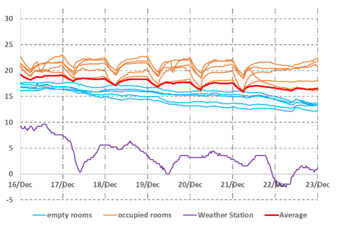
The above graph illustrates an accommodation unit in the week before Christmas when there are no occupants. It is seen that only a fraction of the rooms are heated, as evidenced by the fluctuations in the temperature each morning in some rooms, and the subsequent cooling in the evening (red lines). The blue lines show rooms which continue to cool, but whose temperature is buffered by the red rooms. If none of these rooms are heated, then savings can be or order 10-12% of the total annual heat load.
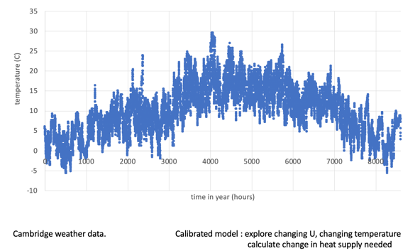
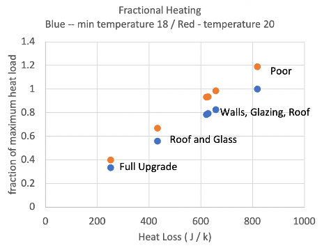
Once we have a calibrated model, we can combine the model with annual weather date, to assess the potential benefits of different energy efficiency measures which would reduce the value of \(U\) (see the 2017 Cambridge temperature data). In the figure below, a series of calculations of the impact of different insulation measures are shown, in terms of the fractional change in heating required over a year, using the Cambridge weather data. The blue curves correspond to a reference temperature of 18C, and the orange show the effect of raising the set temperature to 20C.
These predictions can be tested by comparison with a real upgraded building, as shown in Fig. 10.39 showing gas used in 5 houses in Cambridge. Two of the buildings had substantial improvements in the insulation and the data show this reduced the gas usage by about 50%.
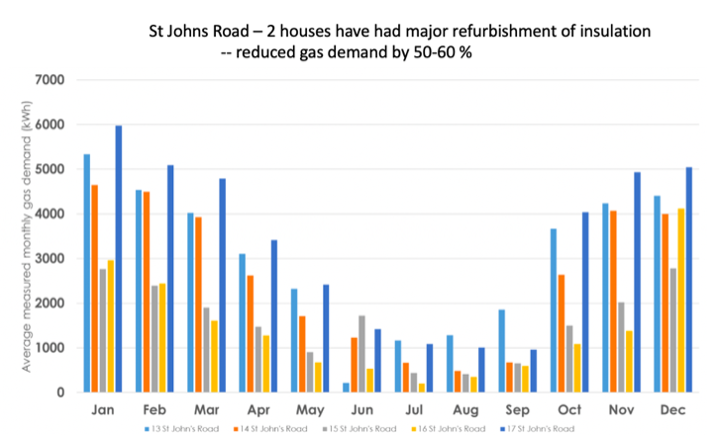
Fig. 10.39 Comparison of gas usage in refurbished and unrefurbished student houses owned by St. John’s college.#