4.4. Reservoirs

Formulation of the reservoir problem

In order to arrest the flow of water from the surface run-off into the river and help mitigate flooding, sometimes reservoirs are built upstream. These lead to accumulation of the surface run-off in the upstream section of the river, and acts as a capacitor in the river system that limits the magnitude of the flow which reaches regions further downstream.

In order to model the effect of a reservoir, we consider a reservoir of area \(A(h)\) when it is filled to height \(h\); a schematic of this is shown in Fig. 4.18.

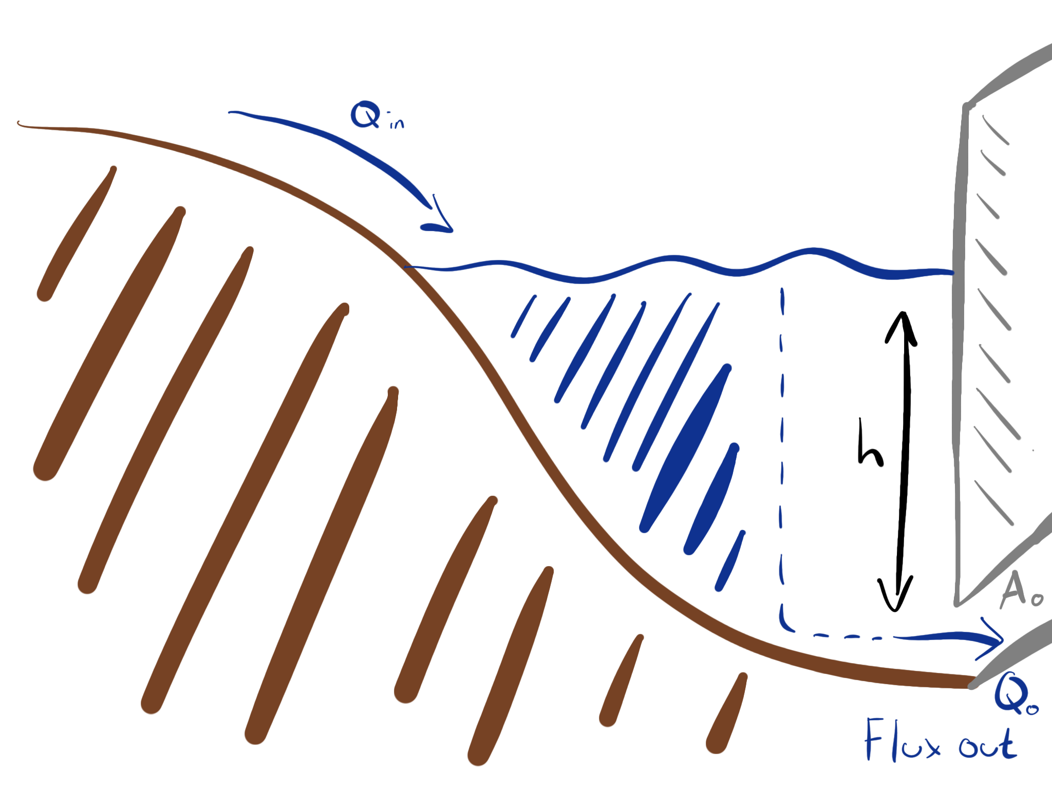
Fig. 4.18 Schematic diagram showing an idealised reservoir. The water is filled up to a height \(h\) and discharges out of the gate of area \(A_0\) at the bottom with a flux \(Q_o\).

Therefore, the volume of water stored in the reservoir is given by

\[V(h) = \int^h_0 A(h')dh'\]

The water in the reservoir flows out of an opening at the base of area \(A_0\), with a speed \(u\). By considering the force of gravity acting on the fluid, we can deduce that the speed of outflow must be

\[u = \sqrt{2gh}\]

and hence the total flux out must be

\[Q_o = uA_0 = A_0 \sqrt{2gh}\]

So, if we assume the upstream waters flow into the reservoir at a rate \(Q_{in}\), then the overall change in the volume of water held in the reservoir with respect to time will be given by

(4.14)\[\begin{split}\begin{align} \dv{V}{t} = &\ Q_{in} - A_0 \sqrt{2gh} \\ = &\ A(h) \dv{h}{t} \end{align}\end{split}\]

At steady-state, we may deduce that, since the volume of water will not change with time, the equilibrium water height in the reservoir is given by

(4.15)\[h_{eq} = \frac{Q_{in}^2}{A_0^2} \frac{1}{2g}\]

With this equilibrium solution in mind, we can now go on to search for a time-dependent solution for \(h\).

Time-dependent solutions for reservoir filling

We will now solve this system for an example reservoir geometry by converting the differential equation to a dimensionless version. This makes our solution easier in the long run because this approach deals with all the constants up front, and will give us a solution that we can analyse the behaviour of, independently of the details of any specific reservoir.

Let us choose the shape of the reservoir such that the area varies as

\[A(h) = \alpha h^2\]

And for convenience we will introduce a dimensionless reservoir depth \(y\), which is relative to the equilibrium height \(h_{eq}\), such that when \(y = 1\), \(h = h_{eq}\).

\[y(t) = \frac{h}{h_{eq}} \quad \tau = \frac{Q_o}{\alpha h_e^3} t\]

We then rearrange the expression of the time dependence of the volume given in equation (4.14) by dividing through by a factor of \(Q_{in}\), which makes the expression dimensionless:

(4.16)\[\frac{\alpha h^2}{Q_{in}} \dv{h}{t} = 1 - \frac{A_0}{Q_{in}} \sqrt{2gh}\]

Substituting the expression for \(y\) into (4.16), it follows that

\[\frac{\alpha (h_{eq} y)^2}{Q_{in}} h_{eq} \dv{y}{t} = 1 - \frac{A_0}{Q_{in}} \sqrt{2gh_{eq}y}\]

and if we recall the expression for the equilibrium height given in (4.15), we can see that the coefficient of \(\sqrt{y}\) on the right hand side is equal to \(1\). So doing some tidying up, we arrive at the expression

(4.17)\[\frac{\alpha h_{eq}^3}{Q_{in}} y^2 \dv{y}{t} = 1 - y^\frac{1}{2}\]

So we now have our equation in a dimensionless form, with a dimensionless “space” coordinate. Our time coordinate, \(t\), however, still has units of time. We therefore want to make a substitution for \(t\) that will replace it with some dimensionless time coordinate \(\tau\). Therefore we make the substitution

(4.18)\[\tau = t \frac{Q_{in}}{\alpha h_{eq}^3}\]

Rationale

This substitution for \(t\) may seem slightly out of the blue. The rationale that one might employ to see that this substitution makes sense when solving this problem ‘out in the wild’ is as follows:

• We wish to find a dimensionless coordinate for time.

• The rest of our equation is already dimensionless, including the space coordinate \(y\).

• Therefore, given that the left hand side of (4.17) is \(\dv{y}{t}\) times some constant, then that constant pre-multiplying that derivative must have units of time if the quantity is dimensionless over all.

• So the reciprocal of that coefficient, multiplied by \(t\), is at least candidate for our substitution.

• What makes it better than any other combination of constants with the units \(\mathrm{s^{-1}}\)?

  • Clearly, it will make the constants out the front of the expression disappear, further simplifying our expression, so it has at least got to be worth a try.

and we will also note that therefore \(T = \frac{\alpha h_{eq}^3}{Q_{in}}\) constitutes some characteristic filling timed for our reservoir. Substituting (4.18) into (4.17) we get

(4.19)\[y^2 \dv{y}{\tau} = 1 - y^\frac{1}{2}\]

This equation can be solved but the algebra becomes involved (use the substitution \(y = (1-s)^2\) ), so we can instead solve the equation numerically, which gives a solution of the form below.

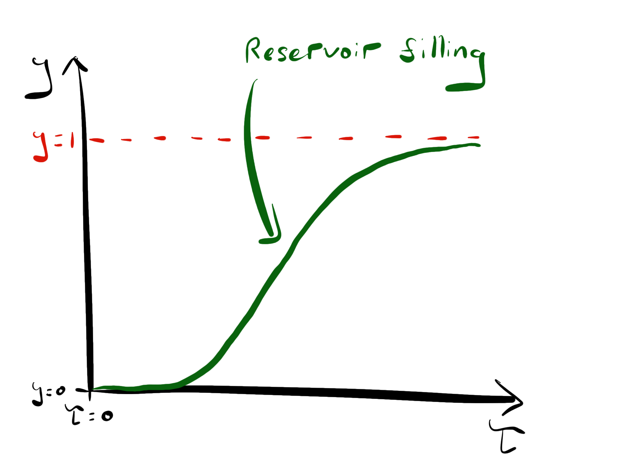
Fig. 4.19 Sketch of the recharge behaviour of a reservoir.

Since \(y\) takes some time to reach equilibrium, the outflow to the river of the full flow from the rain is reduced (until the reservoir fills up).

We can combine this model for a reservoir with the earlier model for the surface run-off to illustrate the effect of the reservoir in buffering the surface run off. An example of this is shown in Fig. 4.20. We combine the model of a rainstorm which leads to an increasing run-off until the rain stops, and then a decaying run-off, as some surface water drains into the ground and the remainder flows into the reservoir.

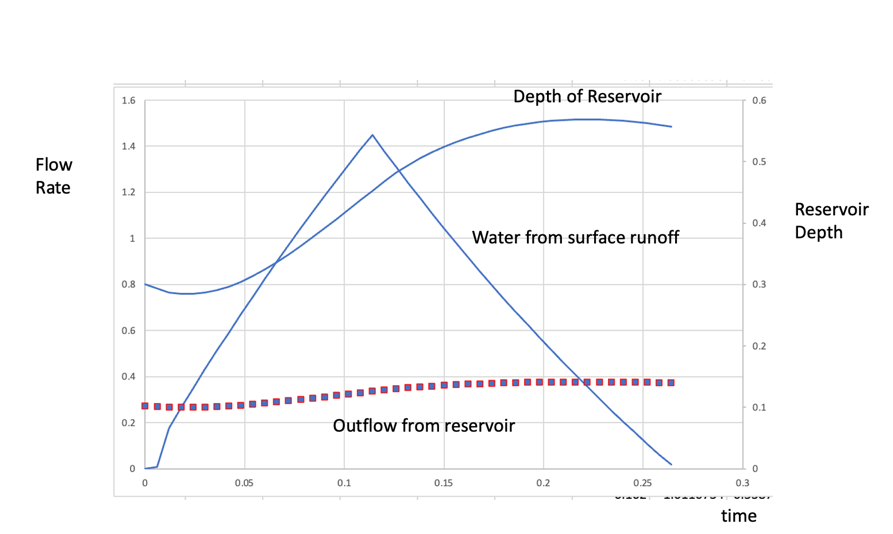
Fig. 4.20 The response of a reservoirs depth, and outflow as a function of the input flow from surface runoff.

Problems with reservoirs: sediment

Rivers globally has a very high sediment load; as such, when a dam is built blocking a river, that sediment accumulates in the reservoir. This has two major effects:

1. The sediment is no longer being sent downstream, so there is ultimately net erosion downstream of the dam.

   • This has the effect of making flooding more likely, as banks are eroded.

   • It also means that the nutrients supplied by the sediment flux are no longer being carried downstream, which can impoverish soil quality.

2. The accumulation of sediment in the reservoir can also reduce the reservoir capacity, by filling up the bottom.

   • This also has an impairs the function of hydroelectric generators, which are often incorporated into reservoir design. The sediment flux can even break the turbines all together.

Resuspension: the Shields criterion

To remove sediment from a reservoir without dredging it, one option is to resuspend the sediment in the flow of water out of the reservoir. In order to resuspend sediment on the bed, the shear force due to the water flowing over it must overcome the weight of the sediment particle.

We therefore relate the shear force, \(F_s\), to the particle diameter, \(d_s\), and densities of the water and sediment, \(\rho_s\) and \(\rho_w\) respectively, given us the Shields criterion for resuspension

\[F_s \gt 0.06 (\rho_s - \rho_w) g d_s\]

where \(0.06\) is an empirical factor, and \(F_s\) is given by

\[F_s = f \rho_w u^2\]

where \(f\) is another empirical factor in the range \(0.01 - 0.1\). Therefore, we need fast flows to resuspend sediment.