3.2. The growth and melting of ice#
The formation of ice in the polar regions is a process central to many ecosystems, to the livelihoods of indigenous and norther communities and, at the largest scales, to the radiative balance at high latitudes. An indication of the extent of the region in the Northern Hemisphere which experiences significant freezing is indicated in the following map of the mean non-frozen days.
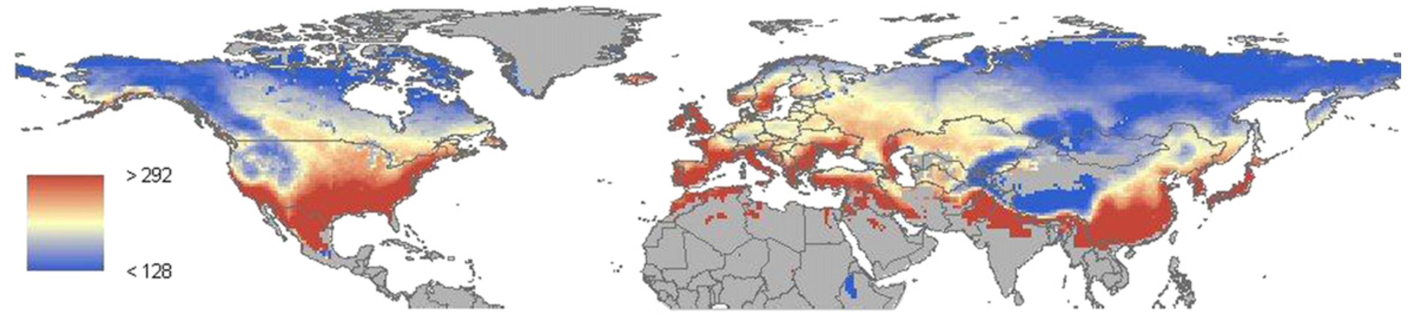
Fig. 3.7 Average number of days per year experiencing non-freezing temperatures in the period 1979-2008 (Kim et al. Remote. Sens. Env. 2012)#
The Stefan problem#
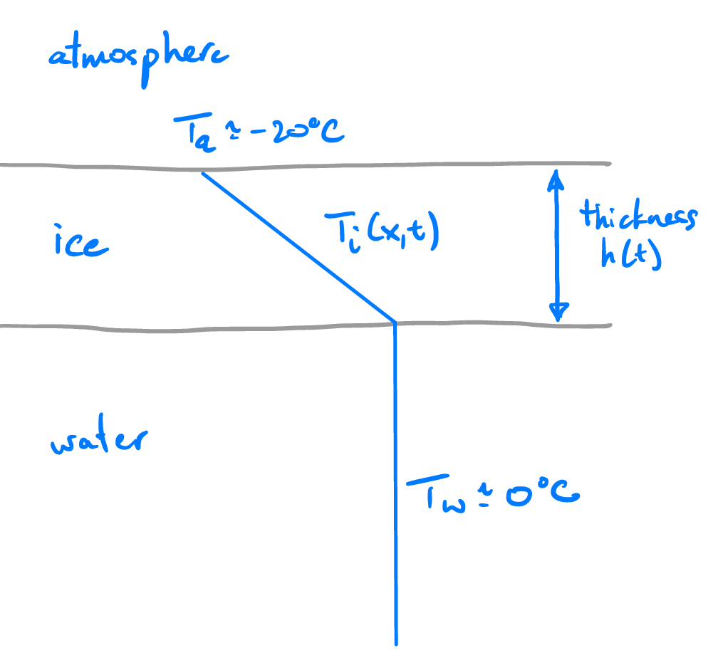
Fig. 3.8 The Stefan problem, in which a layer of ice forms of thickness \(h(t)\) from an upper surface with temperature \(T_a\) into water at the freezing temperature \(T_w\).#
Let’s consider the growth of freshwater ice, and try to predict the thickness of the ice as a function of time. To do so we’ll need to predict the temperature in the ice, and where it reaches the freezing point, \(0~^\circ\mbox{C}\) for fresh (not salty) water, and hence we’ll need to solve for the temperature in the ice, \(T(\mathbf{x},t)\). In general this temperature could depend on both space \(\mathbf{x} = (x,y,z)\) and time \(t\). To start, let’s simplify things by considering a thin layer of ice on a wide body of water so that the temperature is solely a function of the vertical \(T(z,t)\), where \(z\) is the vertical coordinate pointing down into the ice.
The temperature at the surface \(T_s = T(0,t)\) is, in general, set by processes at the surface of the ice. We’ll assume, again for simplicity, that the surface temperature is fixed at \(T_s = -20~^\circ\mbox{C}\). This might correspond, for example, to the arrival of a sudden cold front, or the drop in temperatures as night falls.
The base of the ice is in contact with water, and here the temperature is constrained by phase equilibrium. The phase diagram has the bulk melting point of water at atmospheric pressure to be \(T_m = 0~^\circ\mbox{C}\), so the temperature at the base of the ice \(T_h = T(h,t) = T_m = 0~^\circ\mbox{C}\).
To understand the solidification or melting of any material, ice included, we need to be able to model the flux of thermal energy. To do so we’ll make use of Fourier’s law of heat conduction, which states that thermal energy (heat) flows from a hotter body to a colder one. Hence, in one dimension the vertical heat flux \(F\) in the ice is
where \(k\) is the thermal conductivity which is a material property determining how quickly temperature is conducted the material. For ice \(k \simeq 2.22 \ \mathrm{W \ m^{-1} \ K^{-1}}\), and hence the heat flux \(F\) is measured in \(\mathrm{W \ m^{-2}}\). It is worth noting that, in general, the heat may be written in vector form as \(\mathbf{F} = -k\nabla T\), where \(\nabla = (\pdv{}{x},\pdv{}{y},\pdv{}{z}).\).
The Stefan condition#
The growth or melting of a material requires that sufficient thermal energy is removed or added to drive phase change. At the phase boundary, consider a volume of solid grown per unit area in time \(\Delta t\) is \(v_n\Delta t\), where \(v_n\) is the growth velocity of the interface (measured in the direction normal to the interface). This growth requires an amount of latent heat be removed \(L\rho v_n\Delta t\), where \(L\) is the latent heat and \(\rho\) is the density of the solid. For ice, \(L = 334\ \mbox{kJ kg}^{-1}\) and \(\rho = 917\ \mbox{kg m}^{-3}\). This release / requirement of latent heat (on solidification / melting) must be balanced by the difference in flux of energy over time \(\Delta t\) from the liquid and the solid, \((\mathbf{\hat{n}}\cdot\mathbf{F}_l-\mathbf{\hat{n}}\cdot\mathbf{F}_s)\Delta t\). Hence the general expression for the Stefan condition is
In our two-dimensional system, where the growth rate \(v_n = dh/dt\), this simplifies to
where \(F_l\) and \(F_s\) are the vertical heat fluxes in the solid and liquid respectively.
A first simplified model of ice growth#
Let’s put the pieces together. We’ve made the simplifying assumption that the surface is at fixed (constant) temperature \(T_s\), and we know that the base is at the melting temperature \(T_h = T_m\). While the temperature within the ice is governed by thermal diffusion, let’s make the bold assumption that it is to good approximation linear. Hence the temperature is the ice is approximately,
If the water is initially at temperature \(T_w = T_m\) then the heat flux from the water is zero, \(F_l = 0\). The linear temperature assumption simplifies the Stefan condition to
This is a linear ordinary differential equation for the thickness of ice \(h(t)\), the solution to which is
Here \(\kappa = k/\rho c_p\) is the thermal diffusivity of ice and \(c_p\) is the specific heat capacity. For ice the specific heat capacity, which represents the amount of energy needed to raise the temperature of one kilogram by one degree (Kelvin), is \(c_p = 2.05\ \mbox{kJ kg}^{-1}\mbox{K}^{-1}\) and hence the thermal diffusivity is \(\kappa = 1.2\times10^{-6}\ \mbox{m}^2 \ \mbox{s}^{-1}\). The Stefan number,
is a non-dimensional number which characterises the importance of latent heat release on phase change to the change of temperature within the ice over a characteristic temperature scale \(\Delta T = T_m - T_s\). For the numbers in our example (\(T_m = 0~^\circ\mbox{C},\ T_s = -20~^\circ\mbox{C}\)) the Stefan number \(\mathcal{S} = 8.1\). This is large (\(\mathcal{S} \gg 1\)) and suggests that it is the release of latent heat on solidification that limits the growth of ice.
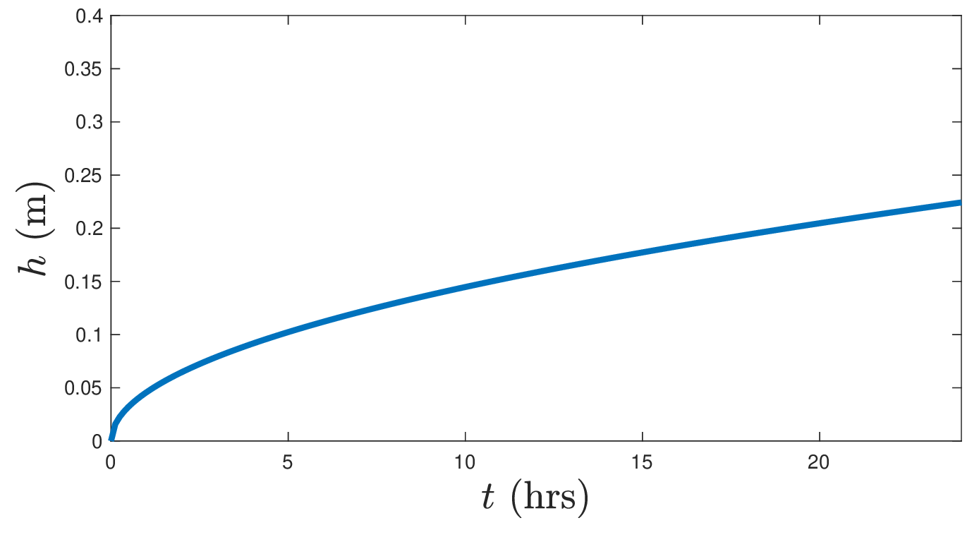
Fig. 3.9 Ice growth from \(T_s = -20~^\circ\mbox{C}\) into water at \(T_w = 0~^\circ\mbox{C}\).#
Our simplified model predicts that ice growth with be rapid at first, and slow down with time as the latent heat of solidification must be conducted through an ever thicker ice cover. This explains why a thin surface skim of ice may rapidly grow on a cold night, but that it takes several days of persistent low temperatures to form a layer you can walk and skate on.
The rapid initial growth of ice also has important implications for the recovery of ice in the polar oceans following the summer melt season. We’ll return to this question in the next lecture, but our result suggests that ice will rapidly regrow following enhanced melting as the climate warms, but that the resultant ice pack may be much thinner.
Forced convection and limits on the growth of ice#
Of course, we’ve simplified the problem greatly, and in many natural settings the water beneath the ice is neither still nor is it at the melting temperature. So long as the atmosphere is sufficiently cold, ice may form on a flowing river, or indeed on a lake before the temperature reaches \(0~^\circ\mbox{C}\). Indeed, since the density of water is greatest at \(4~^\circ\mbox{C}\) lakes typically freeze while the depths are still well above freezing.
Let’s now consider a setting where the water is at \(T_w > T_m\) and the current has a mean speed \(U\) far from the ice-water interface. As described in lecture, we may now anticipate a forced, convective heat flux from the water to the ice of the form,
where \(\lambda\) is a heat transfer coefficient.
The Stefan condition may now be written as
which on using the assumption of a linear temperature profile in the ice becomes
Already it is clear that the ice thickness importantly now reaches a finite thickness as \(t\to\infty\), given by
In fact, with a little more work we can see that at early times as \(h\to0\) we recover our earlier model, since the convective heat flux from the water must be much less than the conductive heat flux through the very thin ice.
In fact, this is still a first order, ordinary differential equation, which we can solve (implicitly) for the ice thickness. We find that
where we have defined the ratio \(\theta = (T_w-T_m)/(T_m-T_s)\) for simplicity of notation.
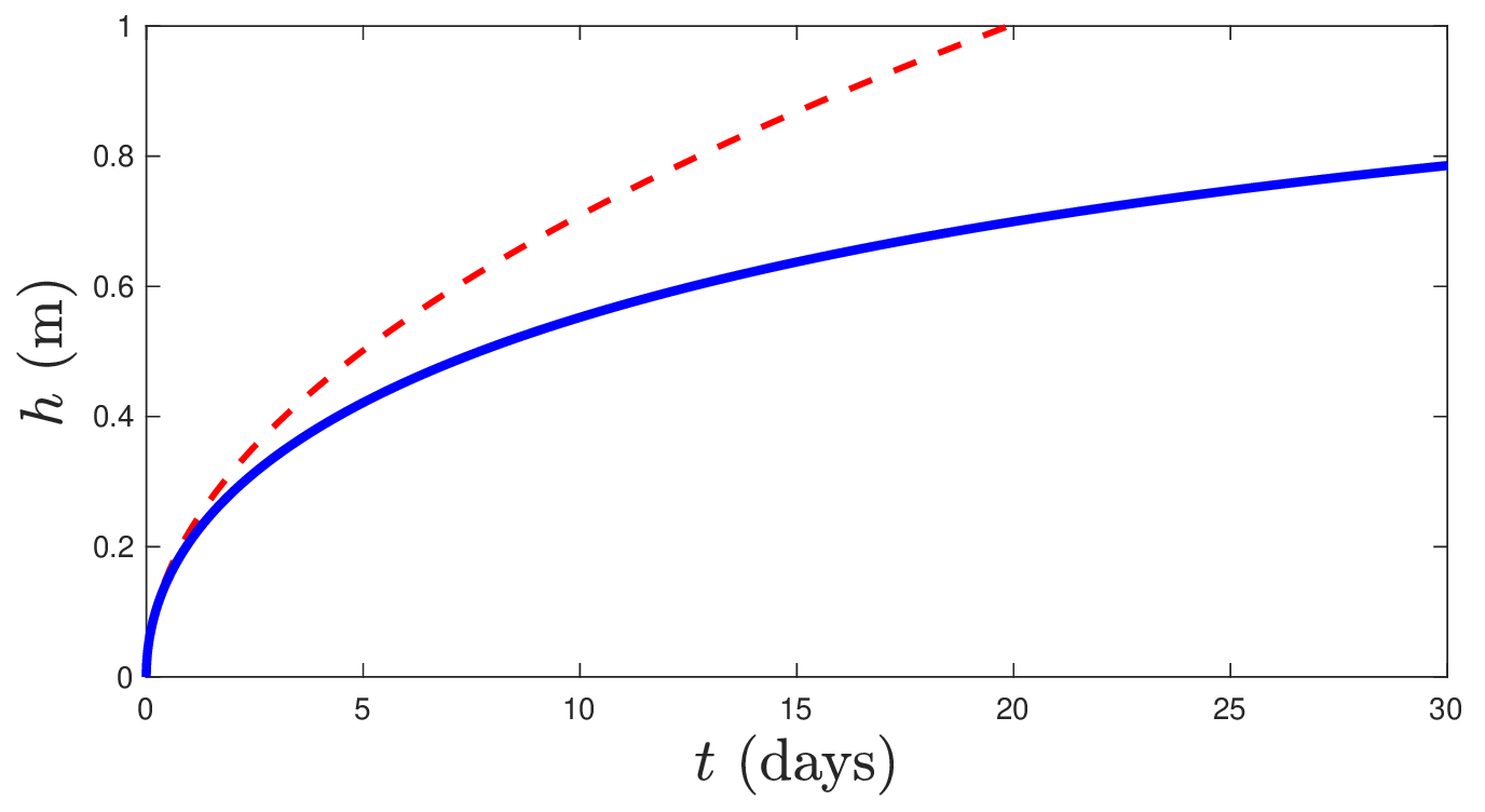
Fig. 3.10 Ice growth from \(T_s = -20~^\circ\mbox{C}\) into water at \(T_w = 4~^\circ\mbox{C}\) and with farfield flow velocity \(U = 1\ \mbox{m/s}\), and with a parameterised heat flux due to the farfield forced flow. Red dashed is the unforced simulation, while solid blue includes the heat flux from the flowing water.#