2.2. Why water moves beneath the surface

Inherent to the idea of a groundwater system is the idea that groundwater moves from a point of recharge to a point of discharge. If the total volume stored is a function of the porosity, then we can ask ourselves what controls how groundwater moves from one point to another point?

This was first explored in the 1850s by Henri D’Arcy, a French civil engineer, who set up a pipe filled with sand and played around with how fast water moved through the pipe.

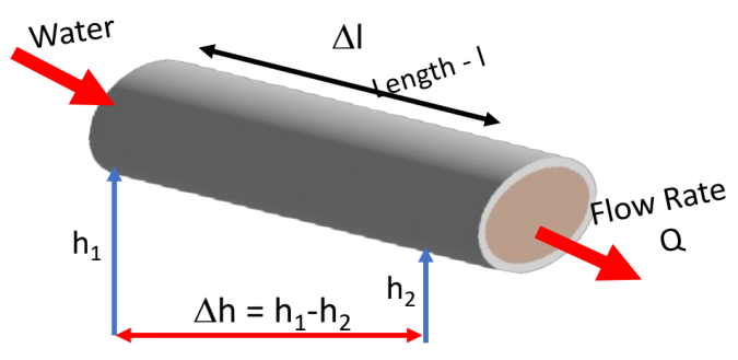
Fig. 2.7 A schematic of the original experiment by Henri D’Arcy.

Units!

\[\begin{split} l, h &= \mathrm{m} \\ Q &= \mathrm{m^3~s^{-1}} \\ \end{split}\]

Here the pipe (length \(l\) and cross-sectional area \(A\)) was put at various angles to the horizontal (determined by \(\Delta h\) – or the height difference between one end of the pipe to the other end of the pipe) and the flow rate, \(Q\), was measured (in units of volume-per-time).

Specifically, we will call \(\frac{\Delta h}{\Delta l}\) – that is the change in height over a distance along the pipe - the hydraulic gradient.

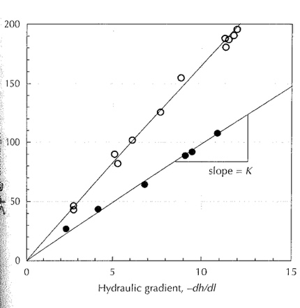
Fig. 2.8 Plot of Flow Rate \((Q)\) against \(-\dv{h}{l}\). The gradient gives \(K\), the hydraulic conductivity.

What Darcy found was that \(Q\) is proportional to \(\Delta h\) and inversely proportional to \(l\). That is the steeper the pipe is held, the larger the volumetric flow rate, and the longer the pipe is the lower the volumetric flow rate. He also found that \(Q\) is proportional to \(A\), that is the larger the pipe, the larger the flow rate. When he filled the pipe with different material, he found that the slope (in a plot of \(Q\) versus \(\frac{\Delta h}{\Delta l}\), Fig. 2.8) changed. He called this slope \(K\) and called it hydraulic conductivity.

Therefore, \(Q \propto - A \frac{\Delta h}{\Delta l}\), which we can turn into an equation using \(K\): \(Q = - K A \frac{\Delta h}{\Delta l}\). Or more generally:

Units!

\[\begin{split} K &= \mathrm{m~s^{-1}} \\ A &= \mathrm{m^2} \\ q &= \mathrm{m~s^{-1}} \\ \end{split}\]

(2.3)\[Q = -KA \dv{h}{l}\]

which is known as Darcy’s law. Note that often you will see \(q\) rather than \(Q\) used where \(q\) is specific discharge, or ‘Darcy velocity’ and is the flow rate (\(Q\)) divided by the area (\(A\)):

(2.4)\[q = \frac{Q}{A}\]

Let’s learn more about this hydraulic conductivity – \(K\). We can derive that the units are length-per-time, or often \(\mathrm{m \ s^{-1}}\). Studies of actual groundwater systems have shown that it can range over 12 orders of magnitude in various materials below the subsurface (Fig. 2.9).

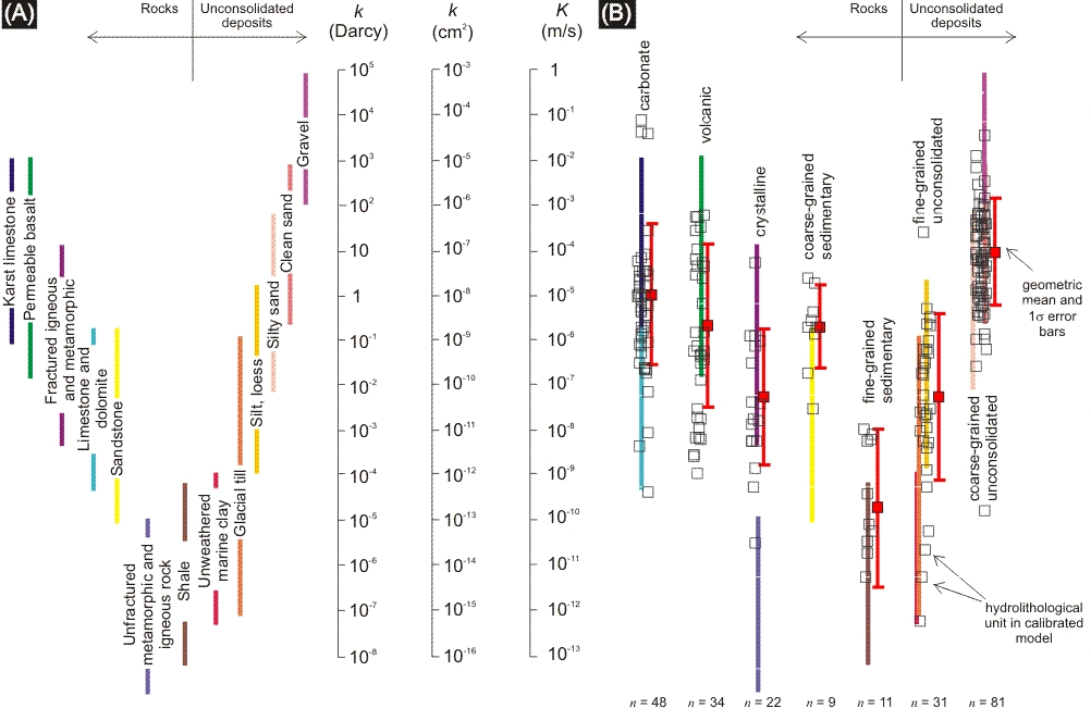
Fig. 2.9 Comparing hydraulic conductivity values from (A) Freeze and Cherry (1979) and (B) calibrayted regional scale hydrogeologic models. Each open square is an optimised or mean value from a part of a model domain that is larger than \(5 \ \mathrm{km}\) horizontally. Values are grouped into hydrolithogic categories that are typical for regioonal-scale modeling (i.e. fine grained, unconsolidated). The geometric meanis shown as a red square with \(1\sigma\) standard deviation for each hydrolithogic category is also shown.

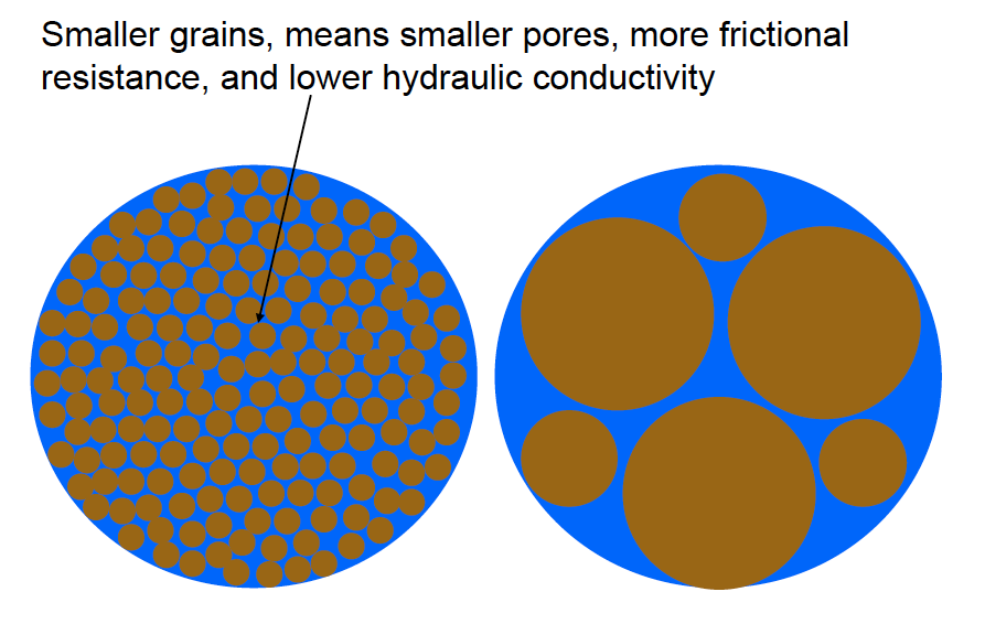
In general, hydraulic conductivity is a function of both the medium (what groundwater flows through) and the fluid that is going through the medium (usually water, in the case of groundwater). \(K\) is:

Units!

\[\begin{split} C &= \mathrm{unitless} \\ \rho &= \mathrm{kg~m^{-3}} \\ g &= \mathrm{m~s^{-2}} \\ \mu &= \mathrm{N~s~m^{-2}} = \mathrm{Pa~s} = \mathrm{kg~m^{-1}~s^{-1}}\\ \end{split}\]

(2.5)\[K = Cd^2 \frac{\rho g}{\mu}\]

Here, \(Cd^2\) is a property of the medium – where \(d\) is the diameter of the grains, and \(C\) is a constant of proportionality, which covers grain packing, how round the grains are, how much cement is around. Meanwhile, \(\frac{\rho g}{\mu}\) is a property of the fluid, with \(\rho g\) being the specific weight of the fluid (\(9800 \ \mathrm{N \ m^3}\)) in the case of water and \(\mu\) being the dynamic viscosity of the fluid (\(1.386 \times 10^{-3} \ \mathrm{N \ s \ m^{-2}}\) for water).

While hydraulic conductivity is a function of the medium and the fluid (imagine trying to put honey through a groundwater system!), in reality, as for most groundwaters the specific weight and dynamic viscosity vary little, what is important is the soil/rock/subsurface (medium) through which you are trying to push groundwater. Mathematically, we call this \(k\) – and it is known as permeability.

Units!

\[\begin{split} k &= \mathrm{m^2} \\ \end{split}\]

(2.6)\[k = Cd^2\]

We can see that we can relate hydraulic conductivity (units \(\mathrm{m \ s^{-1}}\)) to permeability (units \(\mathrm{m^2}\)) quite easily, if we assume that the fluid flowing through the groundwater is water. This is usually a safe assumption (even really salty brines in groundwater systems have a specific weight and dynamic viscosity that means they behave more or less as water). If you read around a bit you will also find that a unit for Permeability of a ‘Darcy’ is sometimes used (but not often).

Fig. 2.9 shows a comparison of hydraulic conductivity from experiments, versus those from hydrology models. This gives you a sense of the hydraulic conductivity associated with different types of material that we find on the surface of the planet. Fig. 2.10 shows a map of the global distribution of permeability which often relates to the underlying rock type. In the lecture we will introduce the concept of Transmissivity, which is the permeability over a particular depth of the aquifer.

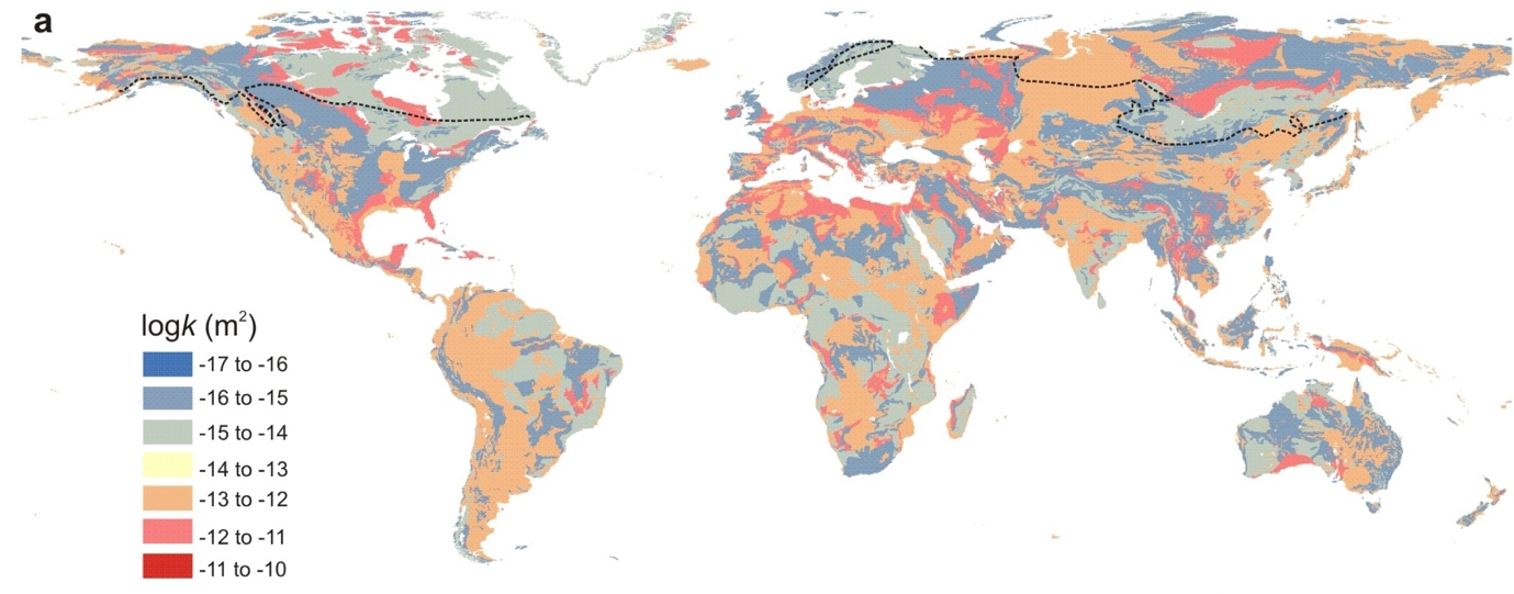
Fig. 2.10 The global distribution of permeability in \(\log(k \ / \ \mathrm{m^2})\). The regional scale permeability will be much lower in the regions north of the dashed continuous permafrost line. Smaller continous permafrost areas in mountainous terrain are not shown.

Darcy’s Law provides us with a nice study of what controls the rate that water flows through porous media. But like all laws it rests on a few assumptions. We need to understand these assumptions before we take the flow through the pipe and translate it to the flow through an actual groundwater system. One of the big assumptions is that flow is laminar, and not turbulent.

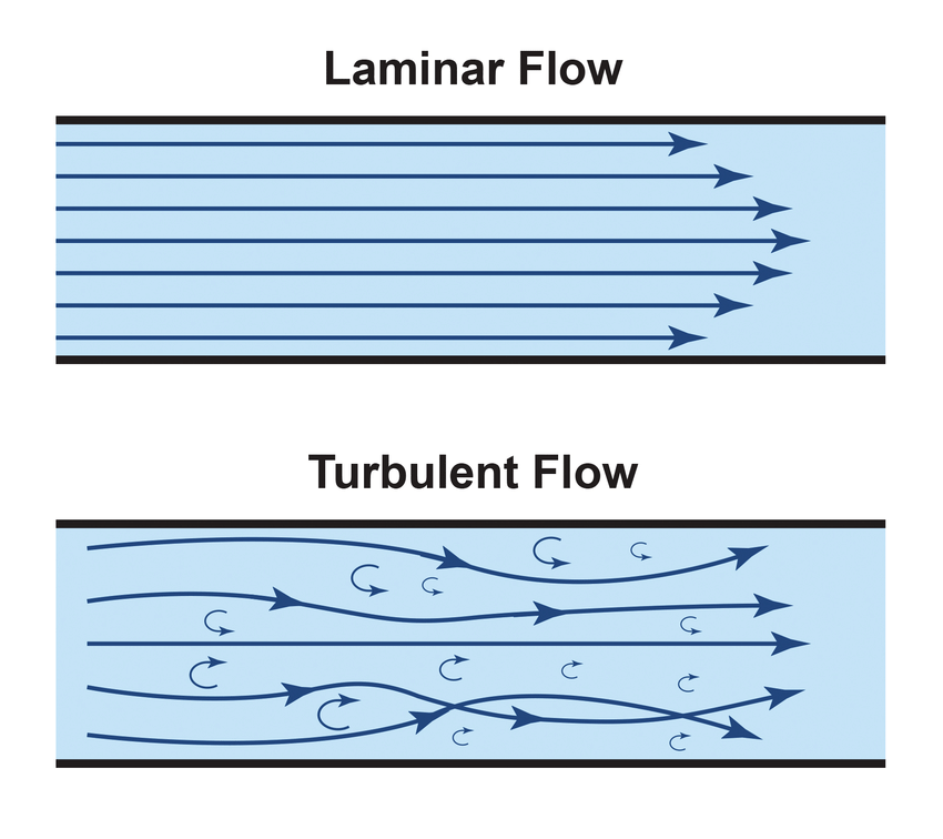
Fig. 2.11 Cartoon of the difference between turbulent and laminar flow.

Laminar means that water is moving in the same direction, like a line, while turbulence occurs when there are deviations from this linearity of movement.

What was seen was that the nice linear relationship inherent to Darcy’s law broke down at high hydraulic gradients, such that \(Q\) no longer scaled linearly with hydraulic gradient.

This is because turbulence has begun in the flow through the porous medium. Turbulence causes pressure loss and thus changes the flow rate.

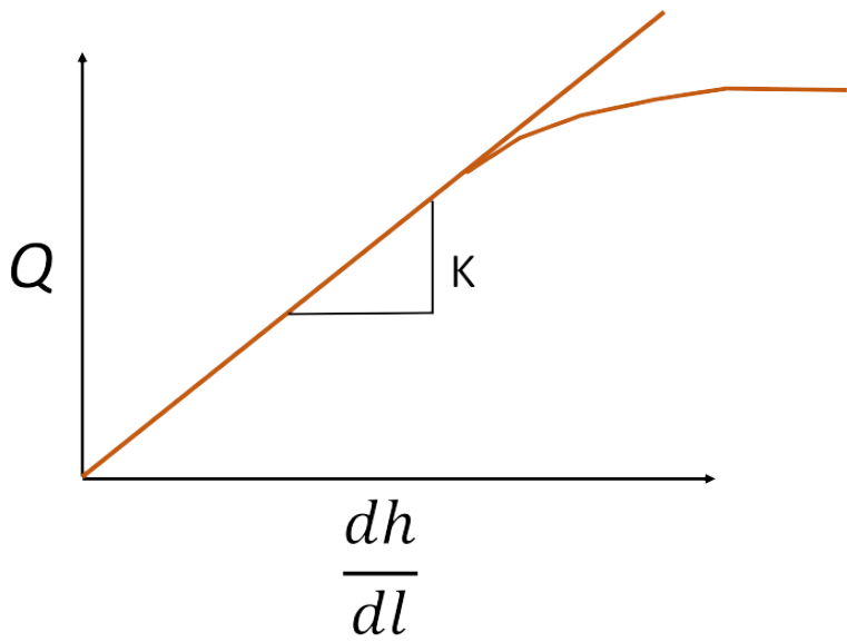
Fig. 2.12 Plot of flow against hydraulic gradient showing the branching of the flow regime. The lower branch represents the turbulent regime, where pressure is lost.

We know if we are in a laminar versus a turbulent flow regime by calculating the Reynolds Number.

Units!

\[\begin{split} \Re &= \mathrm{unitless} \\ \end{split}\]

(2.7)\[\Re = \frac{\rho v d}{\mu}\]

Where \(r\) is the density of the fluid, \(v\) is the velocity of the fluid, \(d\) is a length term, typically the grain size, and \(\mu\) is the dynamic viscosity of the fluid. If \(\mathrm{Re} < 10\) then the flow is laminar, while is \(\mathrm{Re} > 10\) then it is turbulent. Lucky for us, most groundwater systems fall in the category of laminar flow.

Fig. 2.13 Cartoon showing of different porosity materials.

Remember that the grains in the porous media, more generally, provide frictional resistance to the flow. Thus, the velocity of groundwater will be near zero at the interface between the flowing groundwater and the grains, and will be fastest in the middle between the grains. This just means that fundamental properties of the rock/soil/sand have a massive impact on the overall operation of the groundwater system!

Let’s return to groundwater flow. What comes out of Darcy’s law is that the hydraulic gradient, that is \(\frac{\Delta h}{\Delta l}\) drives the flow of water through the pipe, or in case of the real world, the groundwater system. The porous medium (the grains of sand, or sides of the minerals in the rock) resist the flow, providing frictional resistance to the movement of water. The average groundwater velocity is given by \(v = \frac{q}{n}\) where \(q\) is the specific discharge (\(\frac{Q}{A}\)) and \(n\) is the average porosity. The average groundwater velocity \((v)\) is always greater than the specific discharge (remember that porosity is a percentage of void space in the rock!).

We can now think about how this might look in the real world.

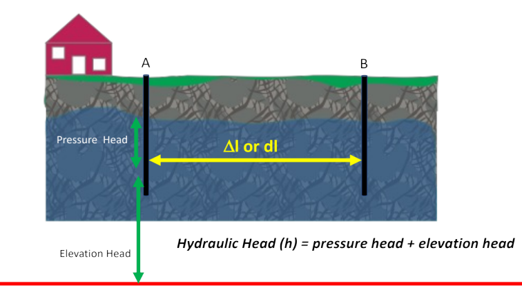
Fig. 2.14 Schematic showing the calculation of hydraulic head.

If we think about a groundwater system, where there are two wells, the pressure of the water at a particular depth in the well is a function of both the pressure exerted by the water above it, and the gravitational pull. Together these are called the hydraulic head. The change in the hydraulic head (\(\dd{h}\) or \(\Delta h\)) over a fixed distance (\(\dd{l}\), or \(\Delta{l}\)) is the hydraulic gradient. This is what drives the water to flow through the porous media (in this case, the rock).

In the lecture we will go through several conceptual models where water flows from high pressure to low pressure, or low pressure to high pressure (canonically flowing ‘up’ or flowing ‘down’) because it is following the gradient of total change in hydraulic head. This means there is a loss of head along the flow-path in a groundwater system. This loss of head amounts to a loss of mechanical energy from the system. But remember, energy must be conserved, it cannot be either created or destroyed. This energy is lost through frictional resistance of the porous media. Here, the loss of energy is lost as heat, as the water squeezes through the rock matrix. The high specific heat capacity of water, however, means that we can’t always measure a change in temperature associated with this conservation of energy!