4.5. Flood waves

We now turn our attention to the propagation of flood waves down a river. This is important to predict since it is useful to know the time of arrival of a flood many tens of kilometers downstream in order to provide warning to residents and try to mitigate the impacts, but also for planning flood prevention systems for example.

We consider a storm that adds an impulse of water to a river of volume \(V\), moving down a river of area \(A\), at a speed \(u\). This gives a flux of water downstream \(Q=uA\). This situation is shown in Fig. 4.21.

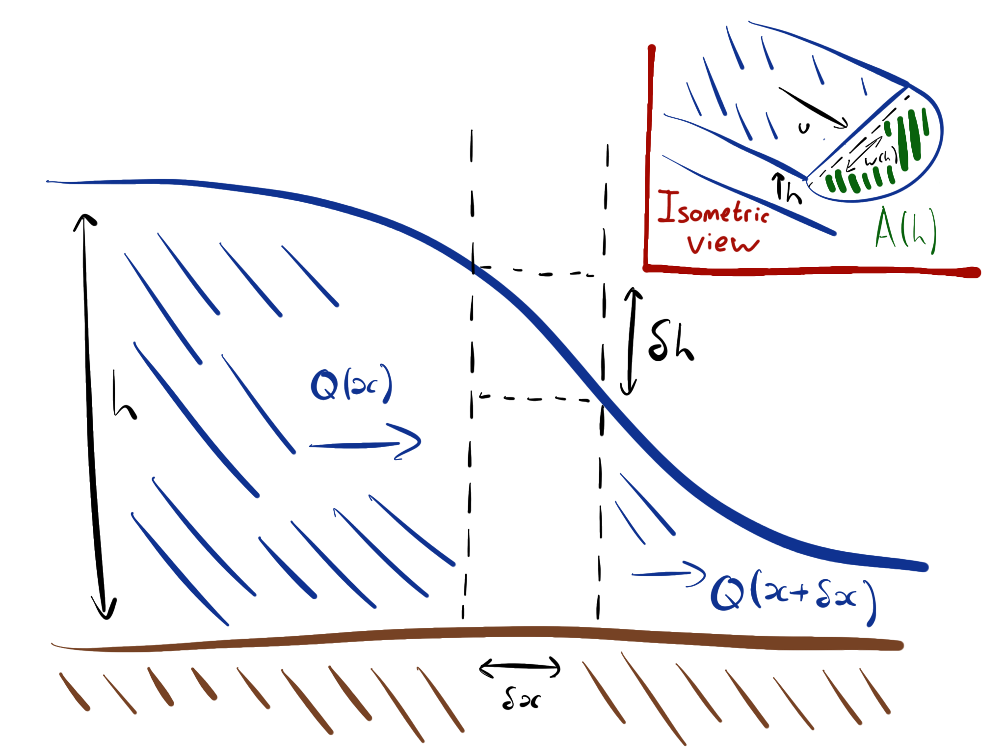
Fig. 4.21 Schematic showing an impulse of water from a storm moving downstream.

If we take the width of the river to be \(W(h)\), then we can relate the change in water volume across a small distance \(\delta x\) to the flux in and out

(4.20)\[\begin{split}\begin{align} W(h) \delta h \delta x = &\ Q(x) - Q(x + \delta x) \delta t \\ W(h) \frac{\delta h}{\delta t} = &\ - \frac{\delta Q}{\delta x} \\ W(h) \pdv{h}{t} = &\ - \pdv{Q}{x} \end{align}\end{split}\]

If we then choose, for the sake of this derivation, a triangular river geometry like that in Section 4.3 where \(A(h) = \alpha h^2\) and \(W(h) = \beta h\). We recall from Section 4.3 that for a triangular river, \(Q = k h^\frac{5}{2}\). we can substitute this into (4.20) by first evaluating \(\pdv{Q}{x}\):

\[\pdv{Q}{x} = \pdv{Q}{h} \pdv{h}{x} = \frac{5}{2} k h^\frac{3}{2} \pdv{h}{x}\]

and with that result now substituting into (4.20)

(4.21)\[\begin{split}\begin{align} \beta h \pdv{h}{t} + \frac{5}{2} k h^\frac{3}{2} \pdv{h}{x} = &\ 0 \\ \pdv{h}{t} + \frac{5k}{2 \beta} h^\frac{1}{2} \pdv{h}{x} = &\ 0 \end{align}\end{split}\]

This analogous to the advection equation we derived in Section 4.2, except this time the characteristic speed \(u\) has been replaced with an expression for the speed that is dependent on the height; \(\frac{5k}{2 \beta} h^\frac{1}{2}\). Therefore, we expect there is a solution for lines of constant height moving down the channel with speed that depends on their depth. Conceptually, this should look like the diagram shown in Fig. 4.22. We are implicitly ignoring the curving over of wave tops that is a familiar feature of breaking waves. This is a very complicated phenomena to model, and doesn’t serve our purposes here to model. We assume that any over-steepened wave instantly breaks, as shown in the lower panel of Fig. 4.22.

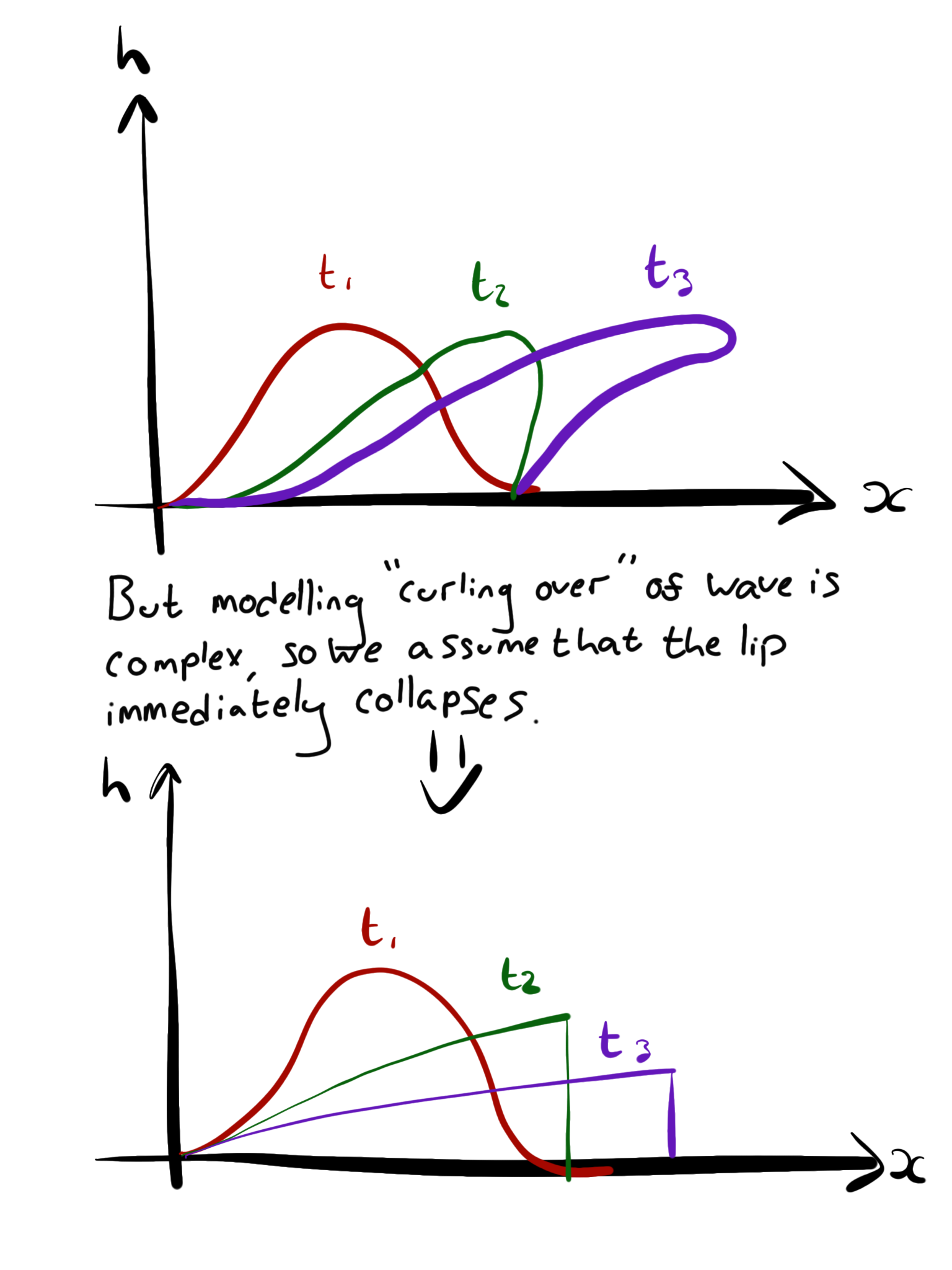
Fig. 4.22 Top: Sketch of the shape of the flood wave nose inferred from the form of the differential equation governing the system. Bottom: Sketch of the shape of the floodwave nose assuming that any over-steepened waves instantly break. The flood wave gets longer and thinner.

We now use the same approach we applied to the advection equation solution in Section 4.2 and try a solution of the form:

\[h(x,t) = Z(x - \frac{5k}{2 \beta} h^\frac{1}{2} t, \tau)\]

i.e. a coordinate change, so that we are now in the frame of reference of the wave (\(\eta\) moves at the speed of a line of constant height \(h\))

\[\eta = x - \frac{5k}{2 \beta} h^\frac{1}{2} t \mathrm{,} \quad \tau=t\]

So then calculating our new derivatives:

\[\begin{split}\begin{align} \pdv{h}{x} = &\ \pdv{Z}{\eta} \pdv{\eta}{x} + \pdv{Z}{\tau} \pdv{\tau}{x} \\ = &\ \pdv{Z}{\eta} \end{align}\end{split}\]

\[\begin{split}\begin{align} \pdv{h}{t} = &\ \pdv{Z}{\eta} \pdv{\eta}{t} + \pdv{Z}{\tau} \pdv{\tau}{t} \\ = &\ \pdv{Z}{\eta} \left(- \frac{5k}{2 \beta} h^\frac{1}{2} \right) + \pdv{Z}{\tau} \end{align}\end{split}\]

Substituting all of this into (4.21) gives us

\[\begin{split}\pdv{Z}{\eta} \left(- \frac{5k}{2 \beta} h^\frac{1}{2} \right) + \pdv{Z}{\tau} + \frac{5k}{2 \beta} h^\frac{1}{2} \pdv{Z}{\eta} = 0 \\ \implies \pdv{Z}{\tau} = 0\end{split}\]

Which means that \(Z\) is constant (i.e. depth is constant) provided we move along a line on which \(\eta\) is constant. So examining one possible solution, for which \(\eta = 0\), we get

\[x = \frac{5k}{2 \beta} h^\frac{1}{2} t \quad \quad h = \mathrm{const.}\]

Rearranging this then gets us to

(4.22)\[h = \left( \frac{2 \beta}{5k} \right)^2 \frac{x^2}{t^2}\]

Using this solution for the long time depth of the current, we can estimate the nose location and depth (see Fig. 4.22 for a reminder of what this looks like).

Applying the conversation of fluid, we first work out the volume in the flow and this leads to an expression for the position of the nose:

(4.23)\[V = \int_0^{x_N} A(h(x,t)) \dd{x}\]

where \(x_N\) is the position of the flood wave nose. We note that

(4.24)\[A = \int_0^{h} W(h') \dd{h'} = \frac{1}{2} \beta h^2\]

and substituting (4.22) and (4.24) into (4.23) we get

\[\begin{split}\begin{align} V = &\ \int_0^{x_N} \frac{1}{2} \beta \left(\frac{2 \beta}{5k} \right)^4 \frac{x^4}{t^4} \dd{x} \\ = &\ \frac{1}{2} \beta \left(\frac{2 \beta}{5k} \right)^4 \frac{x_N^5}{5 t^4} \end{align}\end{split}\]

We can then rearrange to get the nose position as a function of time:

\[x_N(t) = \left[\frac{2}{\beta} \left( \frac{5k}{2 \beta} \right)^4 5V t^4 \right] ^\frac{1}{5} \propto t^\frac{4}{5}\]

and using this nose position we can establish the depth of the flow at the nose to be

\[h_N = \left( \frac{2 \beta}{5k} \right)^2 \left( \frac{x_N}{t} \right)^2 \propto t^{-\frac{2}{5}}\]

which is, interestingly, insensitive to the total volume of water from the storm (\(\propto V^\frac{2}{5}\)).