10.6. Heat pumps#
Although the measures of control and of upgrading insulation discussed in the previous lecture are very important in reducing the demand for heating, there is still a need to decarbonise heating and this can be achieved by replacement of gas with heat pumps. Heat pumps are machines which take heat from a source, then raise the temperature of that heat, and supply the heat to a sink.
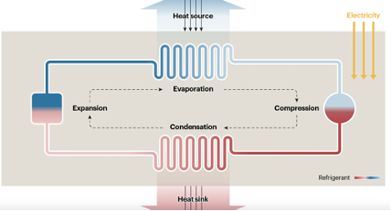
Fig. 10.40 Schematic of a heat pump.#
In order to model the performance of a heat pump we can draw on the ideal Carnot cycle in thermodynamics, which provides a reference for the relationship between the heat supply from a heat pump to the work done and the heat supplied to the heat pump.
The figure of the thermodynamic cycle illustrates the operation of a heat pump in which there are four phases:
A compression phase (C-B) which raises the temperature of the working fluid from the cold side to the hot side of the pump.
A compression phase at constant (high) temperature during which the heat is transferred from the heat pump (B-A).
An adiabatic expansion phase, during which the working fluid cools down as it moves back to the cold side of the heat pump (A-D).
An expansion phase at constant (cold) temperature (D-C) when the heat is supplied to the heat pump from the heat source (which has a temperature higher than this cold side of the heat pump).
In this way, heat is transferred from the cold source to the hot sink by changing the temperature of the working fluid so that (a) it is below the cold source temperature when it takes up the heat from the source and so that (b) it is above the hot sink temperature when it supplies heat to the heat sink. The change in temperature is achieved through the adiabatic expansion and compression, and this requires a net amount of work to be done in moving the working fluid round the heat pump. This work is powered by supplying electricity to the heat pump motor.
The coefficient of performance of the heat pump is given by the ratio of the heat transferred to the hot sink, compared to the work done in achieving this. We now go through the calculation for working out the work done and the heat transfer in an ideal heat pump cycle.
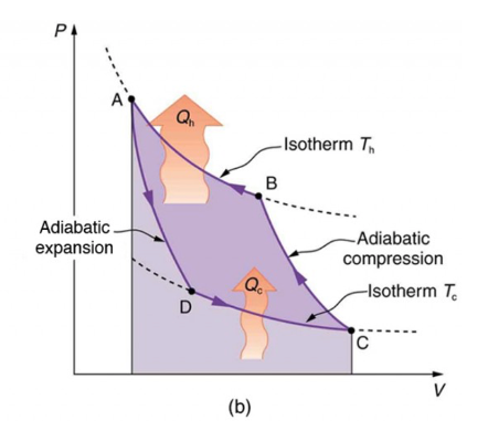
Fig. 10.41 Idealised Carnot cycle.#
We can model each of the 4 phases of the cycle using the 1st law of thermodynamics
where \(\dd{Q}\) is the heat added to the system, \(\dd{U}\) is the change in internal energy, and \(\dd{W}\) is the work done. The work done normally has the form
On the parts of the cycle DC and BA, heat is supplied to the working fluid (DC) or heat is removed from the working fluid (BA), but the temperature of the working fluid remains constant on these two parts of the cycle, and so \(\dd{U} = 0\) and we have
The ideal gas law has the form
And so it follows that
Integrating along BA we have that the change in the properties of the working fluid moving through the heat pump are given by
where \(T_\mathrm{hot}\) is the temperature of the hot side of the heat pump and \(Q_\mathrm{hot}\) is the heat flux provided by the heat pump. Similarly, on the cold side of the heat pump, where the working fluid is cold , \(T_\mathrm{cold}\), and takes in heat \(Q_\mathrm{in}\) from the low temperature heat source
On CB we have adiabatic compression, which raises the temperature of the working fluid, and so
We combine this with the gas law \(PV=RT\) to find a relation between \(T\) and \(V\), which is
This means that on AD
and on CB
Since the temperature is constant on BA,
Similarly the temperature is constant on CD, so
it follows that
And so substituting into eqns (6) and (7), we find that
Finally, energy conservation around the whole ideal cycle requires that
Hence the coefficient of performance, \(\mathrm{CoP}\), is
As an example, if \(T_\mathrm{cold} = 283 / \mathrm{K}\) and \(T_\mathrm{hot} = 313 / \mathrm{K}\), and substituting into eqns (6) and (7), we find that
Non-ideal behaviour of a real heat pump leads to a less efficient system, and typically the CoP is about 3-5 when temperatures are raised from 0-10 C to about 30-40 C. The smaller the temperature increase, the less the work that is needed and hence the higher the CoP.
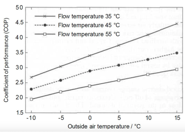
Fig. 10.42 Typical performance data for an air source heat pump#
One key issue with a heat pump is that we need a heat source. There are air source heat pumps which cool the air and if a volume flux \(Q\) of air is cooled by \(\Delta T\), the heat supply to the heat pump is
For \(C\) = 1000 J/kg/K, \(Q\) = 1m3<\sup>/s, \(\Delta T\) = 10, the $Q_\mathrm{in} is about 10 kW.
Ground source heat pumps draw in heat from the ground around a vertical (or horizontal) loop. These supply about 5kW per bore hole, which may be of order 100m deep. Since the heat is supplied to the well through thermal conduction from the ground, the ground around the well gradually cools down as seen in the figure below. Data suggest cooling of about 3K in 5 years. Long term, these need recharging in the summer.
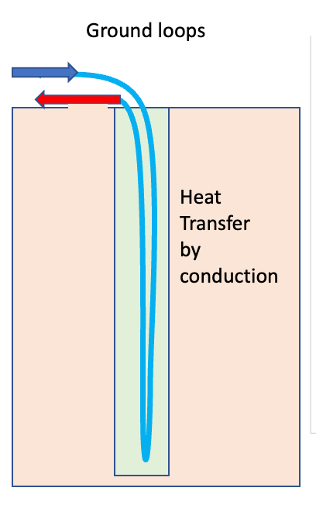
Fig. 10.43 Schematic of a bore hole used to supply energy to a heat pump.#

Fig. 10.44 An example showing where boreholes could be located in St. John’s college. This example shows 120 boreholes on the backs but to meet the college heating demand would require about 800 boreholes.#
With an array of heat pumps, the recovery temperature falls off more quickly since the cooling of each bore hole begins to interfere with the cooling around the next bore hole. For example St Johns needs about 8MW heating on the main college site. With 10 kW boreholes, this requires about 800 – Fig. 10.44 above shows 120 boreholes.
Finally there are water source heat pumps, which draw heat from a lake or river. Given the density of water is 1000 times that of air, and specific heat of water is about 4000 J/kg/K, a flow of about 1.2 l/s cooled by 1 K will supply about 5 kW of heat. The Cam may supply about 10 MW provided the river is not too cold.
The other key issue for heat pump is that there is a need for additional electricity to power the heat pumps. With heat pumps having a CoP of say 3, then the present demand for energy associated with heating will be reduced from 1/0.85 per unit of heating, assuming a gas boiler has an efficiency of 85% in terms of generating heat by burning gas,to 1/3 units of electricity per unit of heat demand. This is a reduction of over a factor of 3. Note that the carbon emissions of electricity are presently about 200 g/kW hr (national average carbon intensity of electricity from the national grid), while the carbon emissions of burning gas are also about 200 g/kWh (including the inefficiency of the boiler). So a heat pump reduces carbon emissions by about 2/3 today. As electricity becomes more decarbonised this reduction will increase.