3.4. Ice sheets and the flow of glacial ice

Glaciers and ice sheets form where ice accumulates persistently over time and compacts to form ice. When the ice is sufficiently thick, the solid ice may flow under its own weight, deforming as a viscous fluid or sliding at the base of the glacier where it contacts the ground or bedrock. Glaciers tend to form at high elevations where it is cold, and snow accumulated in the winter months can persist through the melt season. Their topography is generally determined by the topography (mountains) on which they form.

In contrast, the two major ice sheets on Earth, in Greenland and Antarctica, are so massive that their surface topography is, to a large extent, independent from the topography of the land on which they sit. These massive ice sheets have incorporated a sufficient volume of ice such that they produce their own high elevations and now melt, or are discharged into the ocean, only around their periphery.

In this lecture we will construct models of the flow, accumulation and melting of glaciers in order to understand how glaciers and ice sheets may be expected to respond to climate change.

The viscous flow of ice

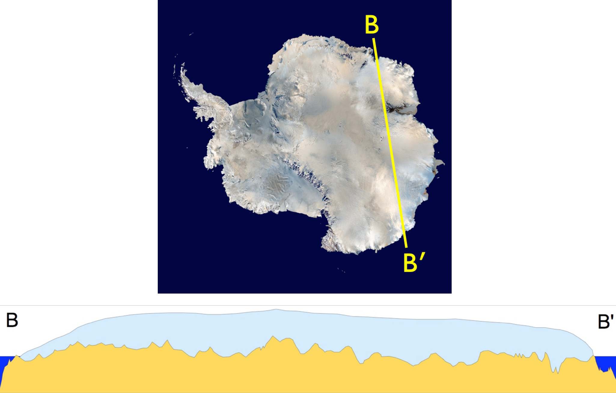
Fig. 3.19 A representation of the long-thin flow of the Antarctic ice sheet over East Antarctica.

The accumulation of ice in Greenland and Antarctica occurs over huge lateral distances of 1000 kilometres or more, with an accumulated depth of 2-3 kilometres (see for example the illustration in Fig. 3.19). Since the lateral extent of the ice is so much greater than the vertical, the flow of ice from the interior to the margins of the ice sheet is predominantly horizontal. Correspondingly, the vertical velocity of the ice is negligible, and the pressure is therefore hydrostatic,

(3.14)\[p = p_0 + \rho g (h-z).\]

Here \(p_0\) is atmospheric pressure, \(\rho\) is the density of the ice, \(g = 9.81\ \mbox{m s}^{-2}\) is the local gravitational acceleration, \(h = h(x,t)\) is the ice thickness which itself may depend on space and time, and \(z\) is the local vertical coordinate (pointing upwards). It is then clear, both from the diagram and from equation (3.14) that there is a pressure gradient from thick to thin regions. It is this pressure gradient which drives the flow of glacial ice, which may be written in the horizontal as

\[\pdv{p}{x} = \rho g \pdv{h}{x}.\]

This pressure gradient is balanced by the viscous resistance to flow of the ice. Viscous resistance is, in general, proportional to the shear which, for long thin ice is predominantly in the vertical, \(\eta \partial u/\partial z\), that shear being proportional to the gradients in the horizontal velocity \(u\) with height \(z\). In the ice sheet, gradients in the horizontal pressure are balanced by vertical gradients in the viscous shear so that

\[\pdv{p}{x} = \rho g \pdv{h}{x} = \eta \pdv{^2u}{z^2}.\]

Since the pressure gradient depends only on \(x\), we can integrate (twice) to find the velocity in the ice

\[u = -\frac{\rho g}{2\eta}\pdv{h}{x} z (2h-z),\]

where we have assumed that the shear at the top surface (\(z = h\)) is zero, and that the velocity at the base (perhaps in contact with the bedrock) is likewise zero. The viscous fluid, ice, therefore deforms with a parabolic velocity profile.

While the velocity of the ice, particularly the surface velocity which may be observed and measured both in situ and remotely, is of interest, it is the mass flux which determines the evolution of the ice sheet and its contribution to sea level rise (for example). Integrating the velocity over the depth therefore gives the mass flux

(3.15)\[q = \int_0^h u\, dz = -\frac{\rho g}{3\eta}h^3\pdv{h}{x}.\]

Locally the mass of ice must be conserved. Hence, the thickness of the ice at any given location is determined by the mass of ice flowing in and out, as well as the rates of accumulation and melting

(3.16)\[\pdv{h}{t} + \pdv{q}{x} = a\]

where here \(a = a(h,t)\) is the accumulation and ablation (or melting) of ice per unit area at a particular location which, in general, depends both on the local elevation and season, and hence depends on time \(t\). A simple model of accumulation and ablation, which makes the mathematical model somewhat easier to solve, is of a constant accumulation / ablation rate above a critical elevation \(h^\star\), which is called the snow line. Let us therefore take the simple model

(3.17)\[\begin{split}a = \left\{ \begin{array}{rl} \alpha & h > h^\star, \\ -\alpha & h < h^\star, \end{array} \right.\end{split}\]

where we take the magnitude of the accumulation / ablation, \(\alpha\), to be a constant (again for simplicity).

Putting together the local statement of mass conservation (equation (3.16)) together with the model for the ice flux (equation (3.15)) and the accumulation/ablation rate (equation (3.17)) we have

\[\begin{split}\pdv{h}{t} - \frac{\rho g}{3\eta}\pdv{}{x}\left(h^3\pdv{h}{x}\right) = \left\{ \begin{array}{rl} \alpha & h > h^\star, \\ -\alpha & h < h^\star. \end{array} \right.\end{split}\]

This is a partial differential equation for the elevation \(h(x,t)\) … but don’t worry, we’ll simplify the equation before attempting to solve it. However, it’s worth noting that for many environmental and climate processes the dynamics depend on space and evolve in time, so a partial differential equation is often the result of such models.

Before we simplify this equation we need to provide some boundary conditions to complete our model. Remember that you need as many boundary conditions as the order of your equation. So for our model we’d need two spatial boundary conditions (though we’ll return to this later), as well as an initial condition.

Since the thickness of the ice may evolve in space and time, we first need an initial condition \(h_0(x) = h(x,t=0)\). We also need a condition at the ice divide, that is at \(x = 0\) in the middle of the continent. Here, there is no input mass flux so we take

\[q(0,t) = \left.-\frac{\rho g}{3\eta}h^3\pdv{h}{x}\right|_{x=0} = 0.\]

If we consider a cross-section of the Greenland ice sheet, much of the ice sheet terminates on land (we’ll consider the ice shelves of Antarctica next lecture). The ice thickness therefore vanishes at the ice edge, or nose, of the ice sheet

\[h(x_N,t) = 0,\]

where \(x_N\) is the position of the nose of the ice sheet measured from the ice divide (so is a measure of the lateral extent of the ice sheet). In this model, we do not know a priori how long the ice sheet may be, and indeed we may want to be able to determine how the ice edge retreats as the climate warms and the elevation of the snow line increases. So \(x_N\) needs to be determined as part of the solution, and therefore we need one last boundary condition. We’ll take that the flux of ice through the nose is zero,

\[q(x_N) = \left. -\frac{\rho g}{3\eta}h^3\pdv{h}{x}\right|_{x = x_N} = 0.\]

This then provides a complete description of our simplified ice sheet model.

The steady state ice sheet

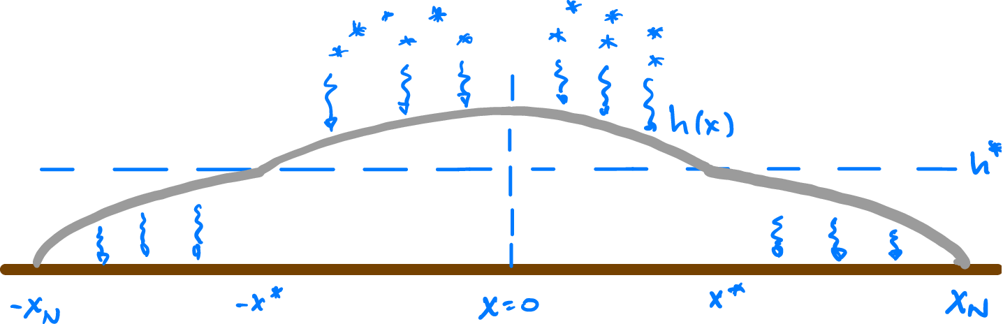
Fig. 3.20 Schematic of the steady-state ice sheet with snow at high elevations (\(h > h^\star\)) and melting at low elevations (\(h < h^\star\)).

To simplify the analysis further, let’s look for so-called steady-state ice sheet models. That is, we’ll seek a solution for the ice sheet in which the net accumulation balances the net melting exactly, and hence the geometry of the ice sheet doesn’t change even as there is a continual flux of ice through the system (this also turns our partial differential equation into an ordinary differential equation!). Hence we take

\[\pdv{h}{t} = 0.\]

First, let’s examine (equation (3.16)), examining above and below the snow line (\(h^\star\)) separately. Above the snow line we solve

\[\pdv{q}{x} = \alpha,\]

and hence, noting that \(q(0) = 0\), we find that

\[q_+ = \alpha x,\]

where the \(+\) indicates the solution above the snow line.

Below the snow line, where the ice is melting, we solve

\[\pdv{q}{x} = -\alpha,\]

and hence, noting that \(q(x_N) = 0\), we find that

\[q_- = \alpha(x_N - x),\]

where the \(-\) indicates the solution below the snow line.

Let’s piece these two solutions together. We know that at the snow line, \(h = h^\star\) at \(x = x^\star\), and that the flux through this point must be continuous. Hence

\[q_+(x^\star) = q_-(x^\star) \quad \implies \quad x^\star = \frac{x_N}{2}.\]

In our simple model for accumulation / ablation, the area of accumulation must be exactly equal to the area of ablation to obtain a steady-state balance.

We can now integrate the expressions for the flux above and below the snow line to determine the thickness of the ice sheet,

\[\begin{split}\begin{eqnarray} h_+^4 & = & \frac{12\eta}{\rho g}\alpha\left(c-\frac{x^2}{2}\right) \quad h > h^\star, \\ h_-^4 & = & \frac{12\eta}{\rho g}\alpha\left(d + \frac{x^2}{2} - x_N x\right) \quad h < h^\star. \end{eqnarray}\end{split}\]

Noting that \(h(x_N) = 0\) gives \(d = 0\), and hence matching \(h_+ = h_- = h_\star\) gives \(x^* = \frac{x_N}{2}\). The complete profile of the ice sheet is therefore given by

\[\begin{split}h = \left\{\begin{array}{ll} \left(\frac{6\eta\alpha}{\rho g}\right)^{1/4} \left(\frac{x_N^2}{2} - x^2\right)^{1/4} & h > h^\star, \\ \left(\frac{6\eta\alpha}{\rho g}\right)^{1/4}\left(x_N^2-2 x_N x + x^2\right)^{1/4} & h < h^\star. \end{array} \right.\end{split}\]

We can determine the lateral scale of the ice sheet, which is set by the material properties of the ice and the height of the now line where \(h(x^\star) = h^\star\), and hence

\[x^\star = \left(\frac{\rho g}{6\eta\alpha}\right)^{1/2}{h^\star}^2.\]

The solution to our steady-state ice sheet model is plotted in Fig. 3.21.

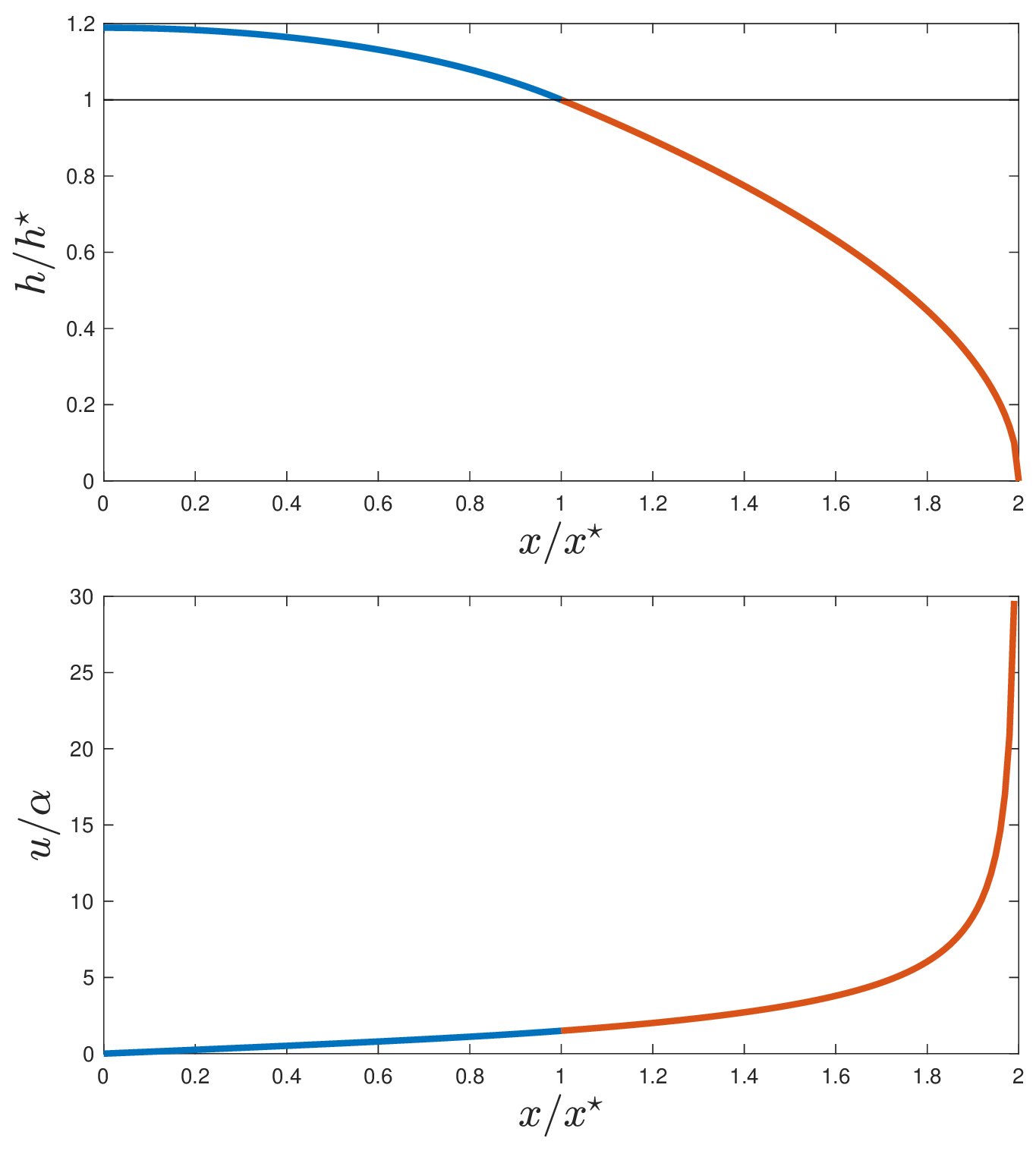
Fig. 3.21 Solution of the steady-state ice sheet model showing (a) the thickness of the ice sheet and (b) the surface velocity.

We have made significant approximations in our model of the steady-state ice sheet, so we shouldn’t expect it to mirror all the features of the large ice sheets exactly. However, the model is able to capture some leading-order features of the Greeland and (East) Antarctic ice sheet. In particular, they mirror the relatively flat interior topography of the ice sheets, with much steeper margins. Correspondingly, the surface ice velocity - which can be measured both by arduous field campaigns or remotely with satellite INterferrometric Synthetic Aperature Radar (INSAR) - shows that ice velocities are relatively low in the interior, but are signficantly higher near the margins where the topographic gradients driving flow are correpsondingly higher. This is reflected, for example, in the map of the surface velocity of the Greenland ice sheet as shown in Fig. 3.22.

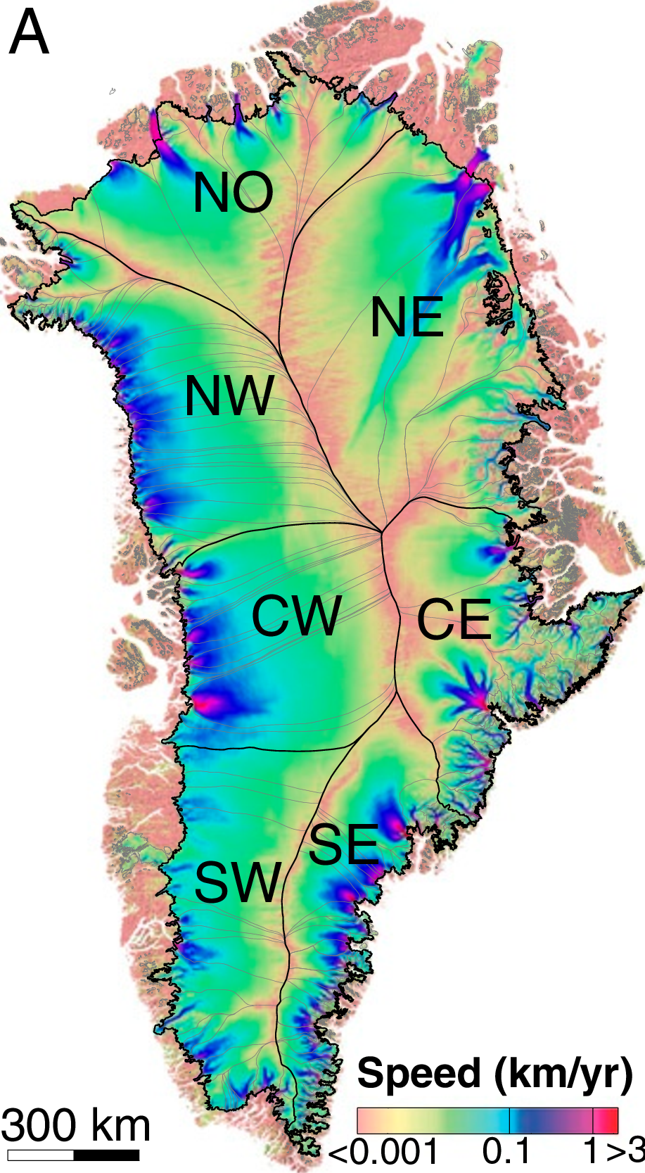
Fig. 3.22 Surface velocity of the Greenland ice sheet from Mouginot et al. Proc. Nat. Acad. Sci. (2019)

Additional processes

Of course the model we’ve just constructed is an intensionally simplified, steady-state ice sheet model with a number of significant pieces neglected. For example, for simplicity we’ve approximated the viscosity of the ice as constant, whereas in practice the viscosity of ice is shear thinning. That is, the ice becomes less viscous the more it is sheared, with a power-law behaviour referred to commonly as Glenn’s flow law. We’ve also assumed that the ice is everywhere stuck to the bedrock, so that the velocity at \(z = 0\) is \(u_b = u(z = 0) = 0\). In practice, as the ice sheet melts around its margins the meltwater is routed to the base of the ice through fractures and moulins in the ice. Water at the base of the ice sheet lubricates the flow of ice, and results in significant basal sliding, \(u_b \neq 0\), with strong seasonal (and even daily) signatures. Finally, it’s worth mentioning that our model of the accumulation / ablation of ice is particularly simplified, and in practice we would expect these rates to depend on distance from the ocean, on elevation, and on the incident solar radiation (as in our previous lectures). Nevertheless, the underlying physical model captures the essential physics and many of these additional processes could be incorporated into a more refined model of the ice sheet.

Finally, our model assumes that the ice sheet terminates on land (\(h(x_N) = 0\)) and in many cases, and particularly in West Antarctica the ice sheet instead flows out onto the ocean as a floating ice sheet. We’ll turn to the dynamics of floating ice sheets in our next lecture, returning to the contribution of ice sheets to sea level changes as we do so.