6.8. Shallow wind-forced ocean circulation#
In the previous section we described a box model for the ocean heat transport. A central feature of this model was a representation of the Thermohaline Circulation (THC) which transports warm water poleward near the ocean surface and returns cold water back to low latitudes in the deep ocean. In the next two sections, we will examine the physical processes that help to set the circulation in the near-surface and deep ocean. Understanding the drivers of the circulation is an important step if we want to understand how the system might change in the future (or how it was different in the past).
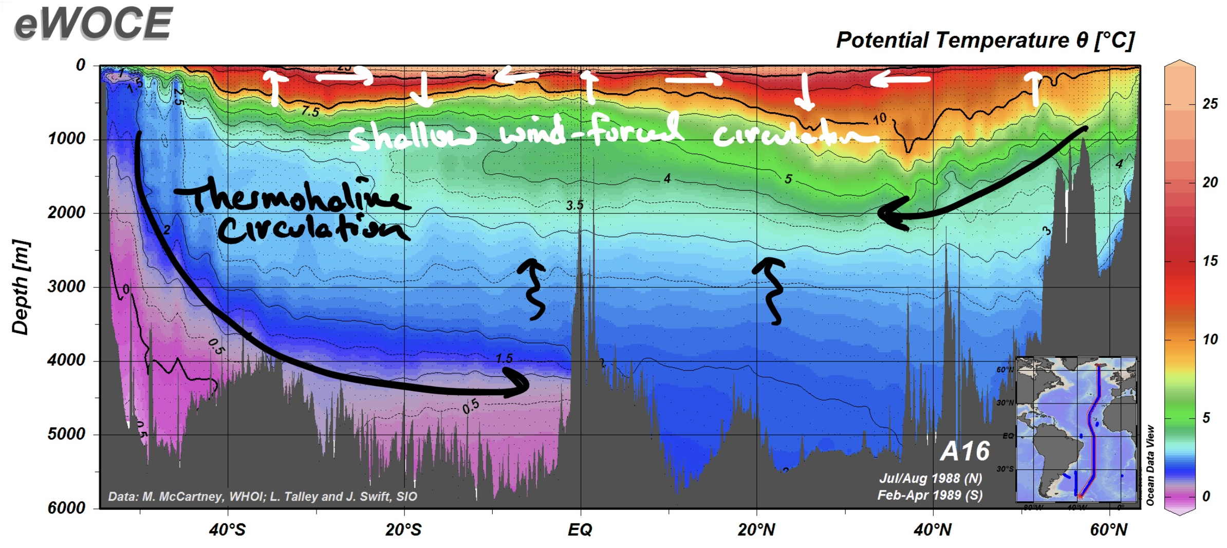
Fig. 6.25 Shallow wind-driven circulation (white) and Thermohaline Circulation (black) drawn on a North/South section from the Atlantic Ocean showing temperature in color and contours.#
Conceptually, we can divide the ocean circulation into shallow wind-forced component and the deep Thermohaline Circulation (THC). Fig. 6.25 sketches these two types of circulation on a temperature section from the Atlantic Ocean as a function of Latitude and depth. In this section we will focus on the shallow wind-forced circulation, and we will discuss the THC in the next section. It is important to note that these two circulation systems are not independent of one another, and despite its name, the Thermohaline Circulation is influenced by wind.
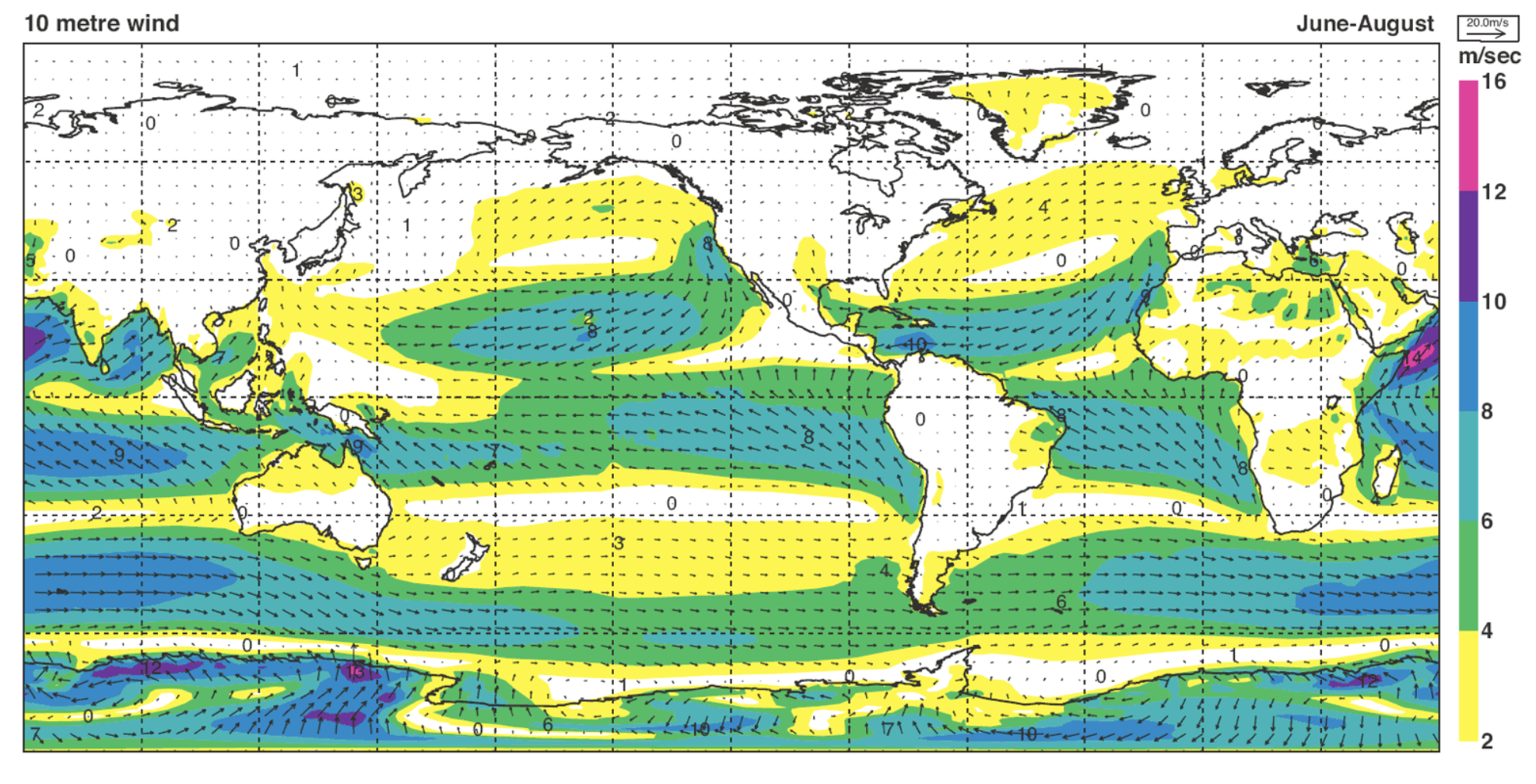
Fig. 6.26 Average wind speed for the months of June - August at a height of 10m. Color shows the magnitude and arrows show the direction. From Kallberg et al. 1995.#
Fig. 6.26 shows the average wind speed and direction at a height of 10m above the ground (or the sea). Note that the wind speed is relatively weak at this height over land due to the extra drag induced by vegetation and topography. The wind patterns that we see in Fig. 6.26 drive the ocean circulation. In particular, both hemispheres have westerly jets (wind coming from the west and going to the east) at mid-latitudes and trade winds in the opposite direction (blowing to the west) at low latitudes. Here, we will refer to the regions between the maxima of the trade winds and the westerly jets as the subtropics. Note that the trade winds are much more pronounced than in Fig. 6.14 since the trade winds are confined to low levels in the atmosphere. Also note that in the Northern Hemisphere summer, the westerly jet in the Northern Hemisphere is weaker than it would be in winter.
When the wind blows over the ocean, it exerts a stress on the ocean surface, and this stress drives currents in the upper ocean. These currents are strongly modified by the Coriolis acceleration, and this has important impacts on the distribution of nutrients and primary production in the upper ocean. We can model the wind stress and study its effects by adding an additional force to our equations of motion. Specifically, the new force will be the derivative of a viscous stress, and the viscous stress is proportional to the vertical derivative of the horizontal velocity where the constant of propotionality is the viscosity \footnote{In reality the stress from the wind is transmitted to the ocean through complicated processes including breaking waves. However, it is common to model this using a viscous stress as we do here, and the mechanism by which the stress is transmitted from the atmosphere to the ocean isn’t critical to the ocean’s response.}. These are the same ideas that we used in the cryosphere lectures.
Specifically, the equations that we will consider are
where \(\nu\) is the kinematic viscosity and has units of length squared per unit time. Note that the last term in Eq. (6.35) only involves vertical derivatives. The full equations also involve horizontal derivatives, but these are typically small compared to the vertical derivatives, so we neglect them.
Since we are interested in the steady-state response of the ocean to wind forcing, we will neglect the time derivative in Eq. (6.35). For simplicity we will also neglect the horizontal components of the pressure gradient. This amounts to assuming that the ocean is uniform horizontally. Then, the horizontal components of Eq. (6.35) are:
Now, let’s integrate these equations in height from a depth, \(z=-h\) to the ocean surface, which we will approximate as \(z=0\) (neglecting surface waves):
The terms on the right hand side can be interpreted as the difference between the viscous stress at \(z=-h\) and \(z=0\). Next, let’s assume that \(z=-h\) is deep enough so that the effects of wind aren’t directly felt and the viscous stress vanishes (we will give a scaling for this depth below). The wind stress \(\mathbf{\tau}^w\) can be represented as the viscous stress at the ocean surface (\(z=0\)):
Suppose that the wind stress is purely aligned with the \(x\) direction, \(\mathbf{\tau}^w=\tau^w \hat{\mathbf{x}}\). Eq. (6.37) then becomes
Remarkably, the depth-integrated velocity in the direction of the wind is zero! Instead, the depth-integrated velocity is directed 90\(^\circ\) to the right of the wind stress in the Northern Hemisphere where \(f>0\).
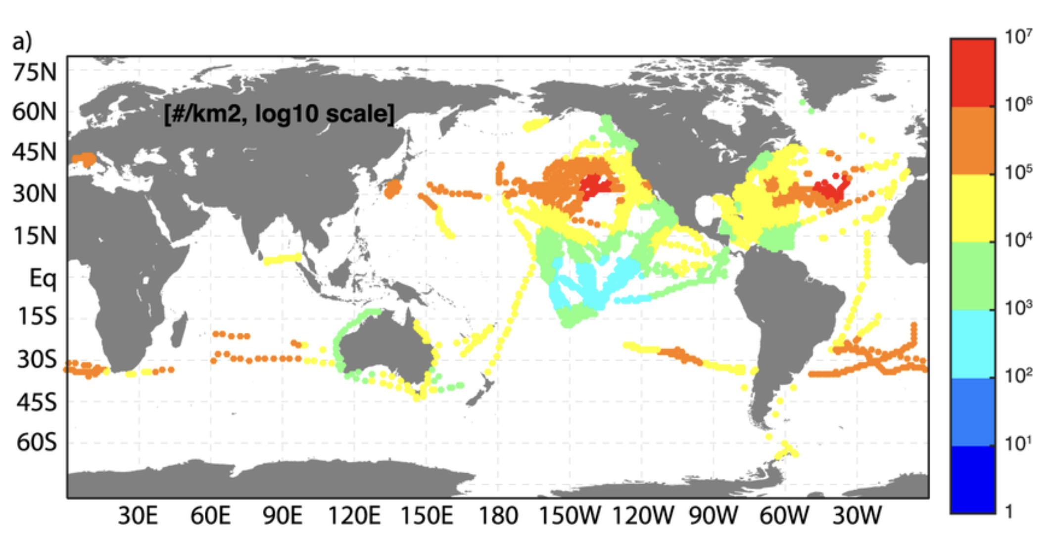
Fig. 6.27 Concentration of microplastics from ship-based surveys. From van Sebille et al.\ 2015.#
In the subtropics, we can see that the wind patterns will lead to a depth-integrated velocity that converges in the middle of the ocean basin. This converging water carries with it floating material which then accumulates in the middle of the ocean basins. This leads to the ‘garbage patches’ that have been observed in the middle of the ocean basins. Fig. 6.27 shows an estimate of the concentration of microplastics based on ship surveys.
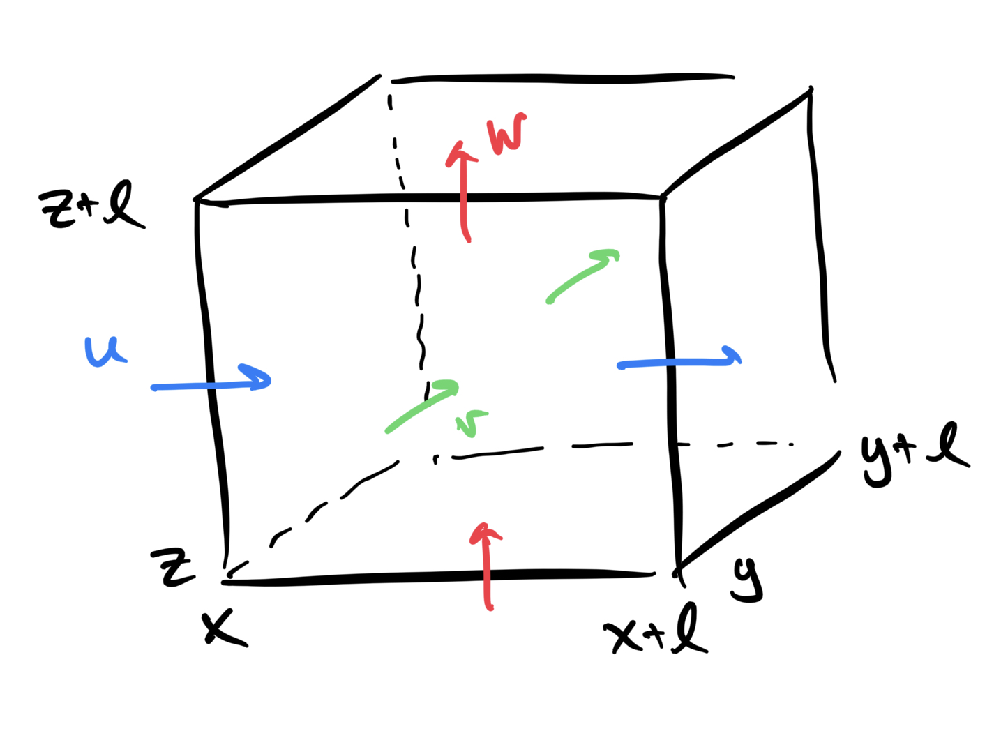
Fig. 6.28 Sketch illustrating volume conservation in a square control volume#
In regions where the wind-forced flow is convergent, the water has to go somewhere and hence the surface waters in these regions move down into the ocean interior. We can show this mathematically by considering a small cube of water as sketched in Fig. 6.28. Let the size of the cube on any single side be \(l\). Let \(x,y,z\) denote the bottom corner of the cube and let \((x+l, y+l, z+l)\) denote the opposite corner. Water can flow in and out of the cube, but to conserve mass, the water flowing in has to be balanced by water flowing out. Hence,
If we move all terms to the same side of the equation and divide by \(l\), we have
If we then take the limit as \(l\rightarrow 0\), we recognize each of these terms as a partial derivative, so that
or in vector form, \(\nabla \cdot \mathbf{u}=0\). This is commonly known as the continuity equation. If we integrate Eq. (6.39) from \(z=-h\) to \(z=0\), we have
Now, let’s apply the continuity equation to the wind-forced flow in the upper ocean. First, since we are considering steady flow on large scales, we can safely assume that \(w(z=0)=0\). In the case when the wind stress is aligned with the \(x\)-direction, we can combine Eqns.\ (6.38) and (6.40) to give
Hence, in the Northern Hemisphere subtropics, where \(\partial \tau^w/\partial y>0\), we have \(w(z=-h)<0\) as we anticipated.
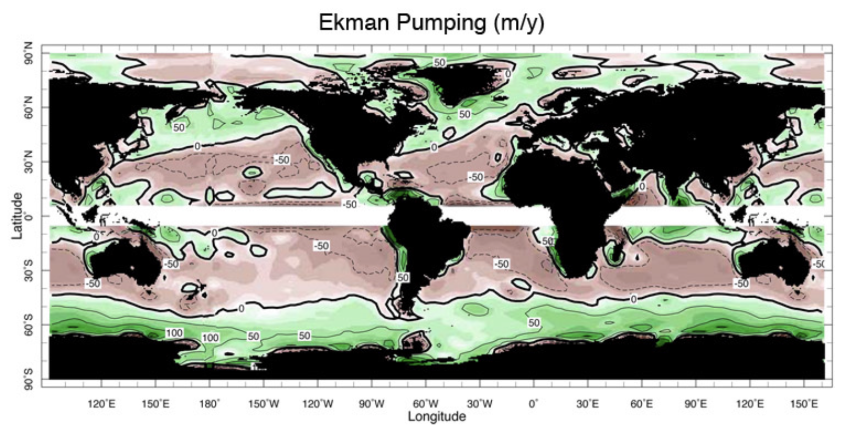
Fig. 6.29 Time-averaged vertical velocity in the upper ocean. Red shading indicates downward motion and green indicates upward motion. The contour labels are in meters per year. From Wunsch, 2011.#
We could extend this analysis for the wind stress vector (without assuming that it is aligned with the \(x\)-axis). Fig. 6.29 shows the time-averaged vertical velocity in the upper ocean (at a depth of about 100m). Comparing with Fig. 6.26, we generally see downwelling in regions where the wind patterns will give a convergent steady circulation, and upwelling where the wind patterns will give a divergent steady circulation.
The downwelling regions in the middle of the ocean basins leads to low biological productivity. Away from the coastlines, microalgae (phytoplankton) growing in the upper ocean tend to deplete the surface waters of essential nutrients. When phytoplankton die, they sink and are eventually broken down by bacteria into inorganic material. This re-supplies nutrients to the ocean interior.
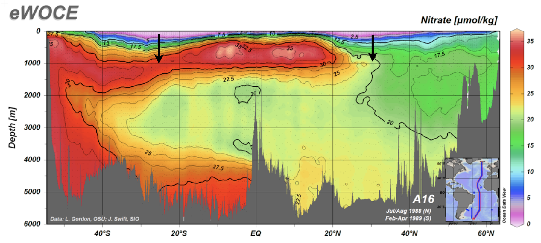
Fig. 6.30 Nitrate concentration as a function of latitude and time for the Atlantic Ocean. The downwelling wind-forced ocean circulation is indicated in black arrow.#
In regions where \(d\tau^w/dy>0\), including the equatorial regions (between the trade winds and the equator) and high latitudes (north of the westerly winds), wind-forced upwelling brings nutrients back to the surface. As a result, these regions are highly productive. On the other hand, when \(d\tau^w/dy<0\), low nutrient water is pushed down into the ocean interior, and the near-surface nutrient concentrations remain low. As a result, these regions have low biological productivity. We can see the tendency for low nutrient waters to be pushed down into the ocean interior in Fig. 6.30 which shows nitrate (an important nutrient) on a north/south section of the Atlantic.
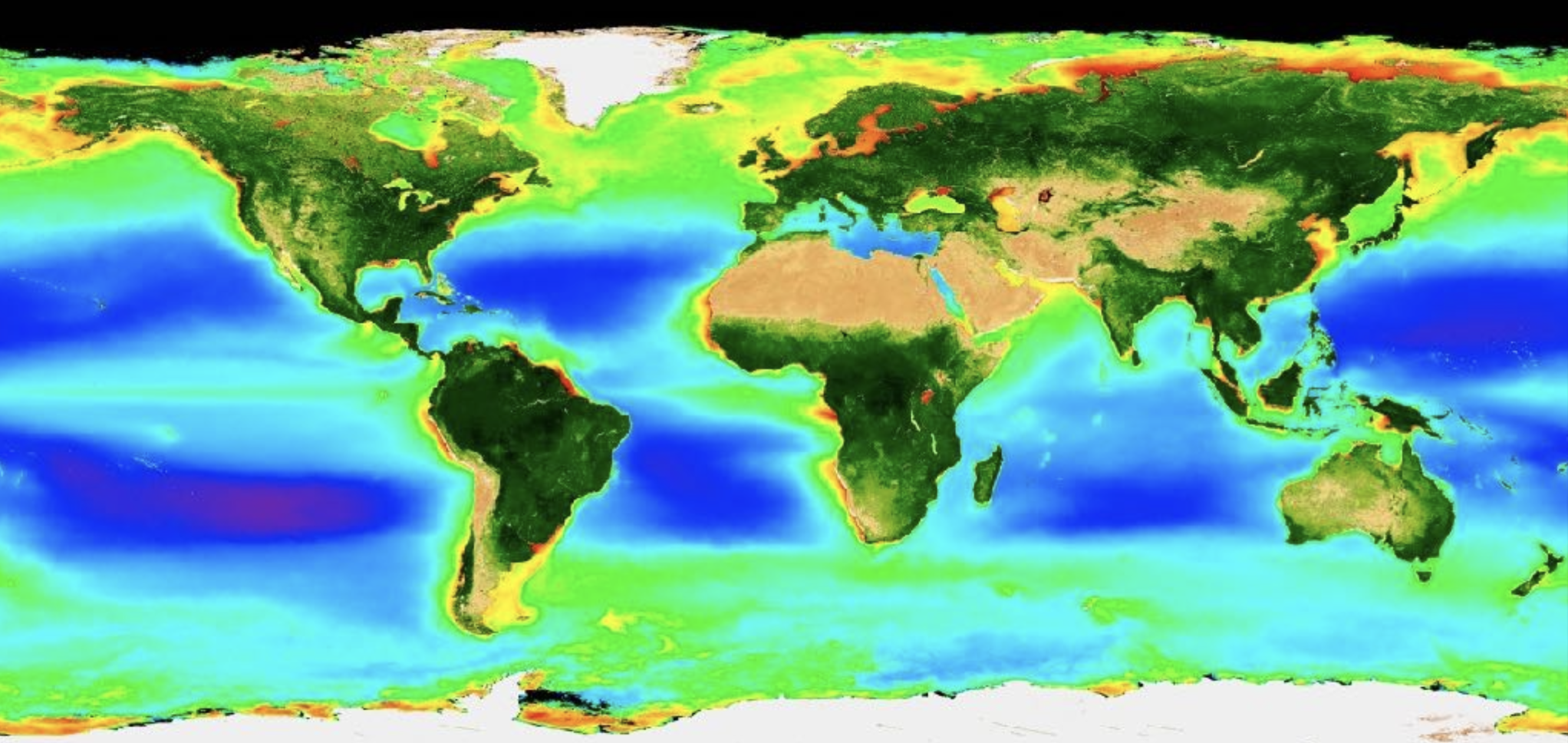
Fig. 6.31 Mean (time-averaged) near-surface chlorophyll concentration inferred from an ocean color satellite.#
Fig. 6.31 shows a time-average of the near-surface chlorophyll concentration inferred from an ocean color satellite. This is plotted using a logarithmic colorbar where green is about 10 times larger than blue and red is about 10 times larger than green. The patterns of high and low chlorophyll are generally what we would expect based on the influence of the wind-forced circulation described above.
Finally, let’s use a scaling analysis to estimate the depth over which the wind forcing penetrates. Let \(U\) be a characteristic horizontal velocity and \(H\) be a characteristic vertical length scale (which we ultimately want to find). Eq. (6.35) then suggests that
or
The kinematic viscosity of seawater is about \(\nu=10^{-6} \mbox{m}^2/\mbox{s}\). If we use \(f=10^{-4} \mbox{s}^{-1}\) which is characteristic of mid-latitudes, then we have \(H\simeq 10\)cm. In reality, the wind-forced circulation is much deeper than this. Instead of molecular viscosity, momentum is carried down by turbulent eddies. We can estimate this like we did in the atmosphere lectures by invoking a turbulent viscosity, which scales as the product of a turbulent velocity scale, \(u^*\), and the length scale, \(H\) (assuming that the size of turbulent eddies matches the size of the wind-forced layer) such that \(\nu_t\sim u^*H\). If we use this scaling in Eq. (6.41), we get
Solving for H gives \(H=u^*/f\). We can get an expression for the velocity scale by noting that the units of \(\tau^w/\rho\) are
and hence \(U\sim \sqrt{\tau^w/\rho}\). Using this in our scaling for \(H\) gives
Fig. 6.32 Mean wind stress magnitude over the surface of the ocean. From Cronin and Tozuka, 2016.#
Fig. 6.32 shows a map of the time-averaged wind stress magnitude. A typical value is \(\tau^w \simeq 0.1 \mbox{N}/\mbox{m}^2\). If we also use \(\rho=1000 \mbox{kg}/\ mbox{m}^3\) and \(f=10^{-4} \mbox{s}^{-1}\), then we have \(H\simeq 100\)m. This is a typical number for the depth of the wind-forced ocean circulation. Note that this is shallow compared to the full depth of the ocean in most places. In the next section we will examine the deeper Thermohaline Circulation.