6.2. Equations of motion on the rotating earth

The Earth’s rotation is an important factor in the large-scale dynamics of the atmosphere and ocean. In this section, we will start to examine the influence of the Earth’s rotation on the equations for fluid motion. To start, let’s consider the acceleration of a point mass in a rotating reference frame.

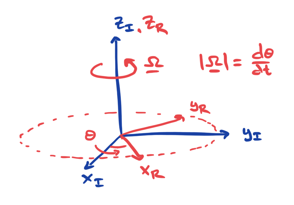
Fig. 6.8 Sketch of rotating and inertial reference frames.

Consider a reference frame rotating about the \(z\) axis with a constant angular velocity, \(\mathbf{\Omega}=\Omega \hat{\mathbf{z}}\). Here, bold symbols will be used to denote vector quantities. Let subscript \(I\) denote a quantity in an inertial (non-rotating) reference frame, and let subscript \(R\) denote a quantity in the rotating reference frame. Fig. 6.8 illustrates rotating and non-rotating reference frames.

A point that is stationary in the rotating reference frame will move in the inertial reference frame with a velocity \(\mathbf{\Omega} \times \mathbf{x}\), where \(\times\) denotes the vector (or cross) product. Therefore, for a point with position vector \(\mathbf{x}_R\) that is moving with a velocity \(\mathbf{u}_R\) in the rotating reference frame, its velocity in the inertial reference frame will be :

(6.1)\[\mathbf{u}_I=\mathbf{u}_R + \mathbf{\Omega} \times \mathbf{x},\]

or the sum of the velocity vector associated with the movement of the rotating reference frame and the velocity of the point in the rotating reference frame.

Note that the velocity vector can be found by taking the time-derivative of the position vector, i.e. \(\mathbf{u}=d\mathbf{x}/dt\),and Eq. (6.1) can be written

(6.2)\[\left.\frac{d\mathbf{x}}{dt}\right|_I=\left.\frac{d\mathbf{x}}{dt}\right|_R + \mathbf{\Omega} \times \mathbf{x}. \]

From this equation we see that the time-derivative of a vector \(\mathbf{x}\) in the inertial reference frame can be written as the sum of the time-derivative of a vector \(\mathbf{x}\) in the rotating reference frame and the vector (cross) product of the angular velocity and the vector \(\mathbf{x}\). If this holds for the vector \(\mathbf{x}\), then it should (and does!) hold for any other vector. We can therefore use this rule to find an expression for the acceleration in the inertial reference frame. Using Eq. (6.1), we find that the time-derivative of the velocity in the inertial reference frame is

(6.3)\[\begin{split}\left.\frac{d\mathbf{u}}{dt}\right|_I&=\frac{d}{dt}\left.\left(\mathbf{u}_R + \mathbf{\Omega}\times \mathbf{x}\right)\right|_R + \mathbf{\Omega} \times (\mathbf{u}_R + \left.\mathbf{\Omega}\times \mathbf{x})\right|_R \\ &=\left.\frac{d\mathbf{u}}{dt}\right|_R + 2 \mathbf{\Omega} \times \mathbf{u}_R + \mathbf{\Omega} \times (\mathbf{\Omega} \times \mathbf{x}),\end{split}\]

where we have assumed that \(\mathbf{\Omega}\) is constant. The last two terms in Eq. (6.3) are the Coriolis acceleration and the centrifugal acceleration. The centrifugal acceleration points radially outwards from the axis of rotation. The corresponding force, the centrigual force is the apparent force that you feel when a car turns suddenly, or on the flying swings or other spinning amusement park rides.

Curiously, the Coriolis acceleration is perpendicular to the velocity of the point in the rotating reference frame (recall that if \(\mathbf{a}=\mathbf{b} \times \mathbf{c}\), then \(\mathbf{a}\) is perpendicular to both \(\mathbf{b}\) and \(\mathbf{c}\)). This property of the Coriolis acceleration leads to some non-intuitive properties of large-scale motion in the atmosphere and ocean.

The movement of air in the atmosphere and water in the ocean is subject to a force induced by gradients in pressure. The sense of the pressure gradient force is to push fluid from regions of high pressure towards regions with low pressure. We encountered this force last term when discussing the cryosphere. The pressure gradient force also causes ice to flow away from regions with high pressure.

We can write an expression for the acceleration of a fluid (air or water) due to a pressure gradient in a {non-rotating} reference frame using Newton’s second law:

(6.4)\[\rho\frac{\partial \mathbf{u}}{\partial t} = - \nabla p.\]

Note that this equation has units of force per unit volume. The pressure, \(p\), has units of force per unit area, and the density, \(\rho\) has units of mass per unit volume.[1] Therefore, the right hand side of Eq. (6.4) is the force per unit volume, and the left hand side is mass per unit volume times acceleration. We can write the equivalent equation in a rotating reference frame using Eq. (6.3):

(6.5)\[\rho\left[\left.\frac{d\mathbf{u}}{dt}\right|_R + 2 \mathbf{\Omega} \times \mathbf{u}_R + \mathbf{\Omega \times (\mathbf{\Omega \times \mathbf{x})}}\right] = -\nabla p.\]

From this point on, we will exclusively consider a rotating reference frame (the Earth) and will drop the subscript \(R\).

If the atmosphere and ocean were at rest (with \(\mathbf{u}=\mathbf{0}\)), then the only non-zero term on the RHS of Eq. (6.5) would be the centrifugal acceleration which would then balance the pressure gradient. On the rotating Earth, the centrifugal acceleration causes the atmosphere and ocean to bulge outwards at the equator, away from the axis of rotation. The interior of the Earth is also fluid, and hence the surface of the Earth similarly bulges outwards at the equator. In fact, the Earth’s radius at the equator is 22km larger than the radius at the poles. The radial displacement relative to these slightly bulging surfaces is called geopotential height. On surfaces with constant geopotential height (e.g. the surface of a stationary ocean), the outward centrifugal acceleration is balanced by the inward pull of gravity. Since flows in the atmosphere and ocean tend to move along surfaces with constant geopotential height, the centrifugal acceleration plays a relatively minor role in atmosphere/ocean dynamics.

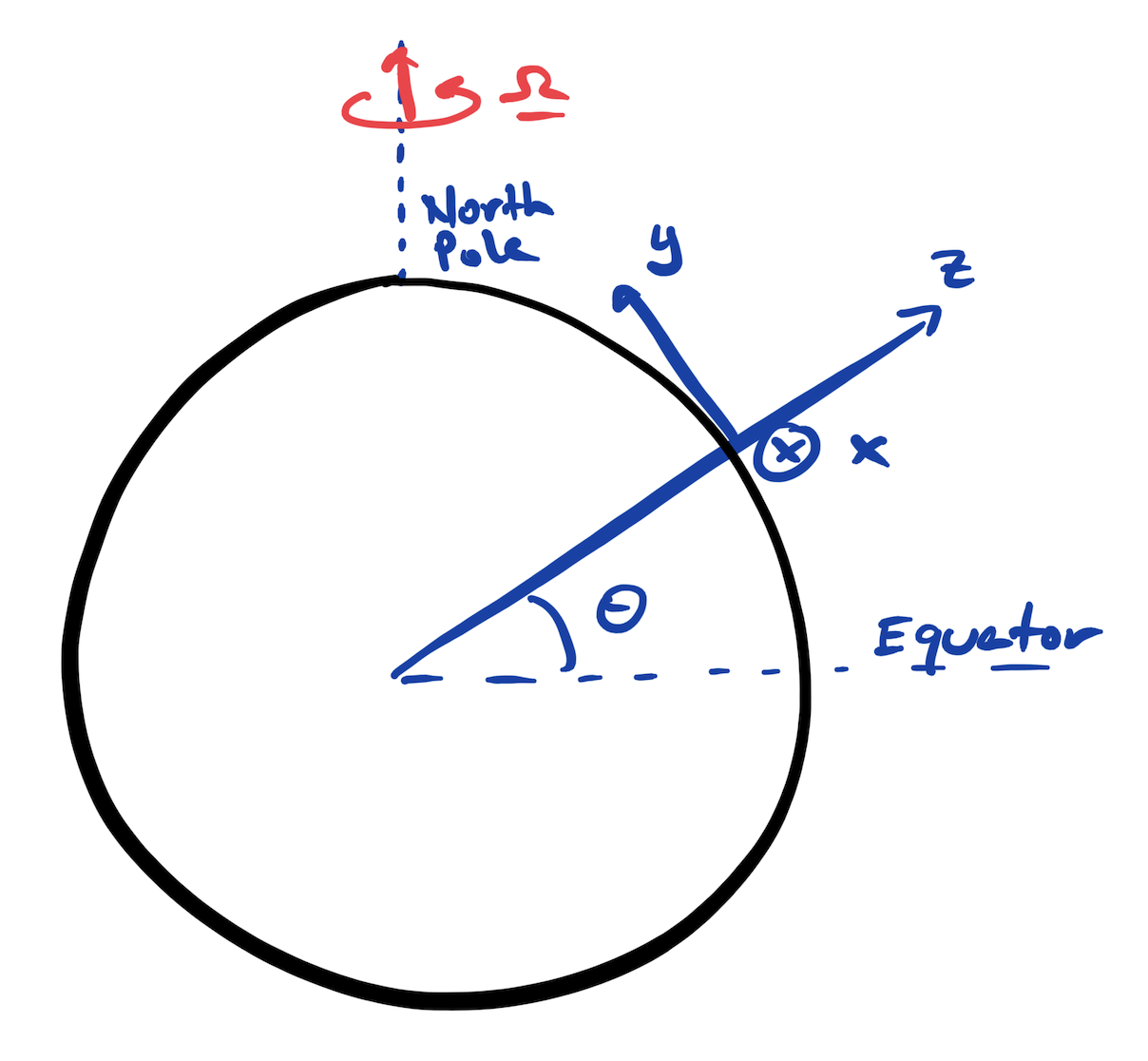
Fig. 6.9 Sketch of a local Cartesian coordinate system

Since writing equations in geopotential coordinates is cumbersome, when studying motion that is small compared to the radius of the Earth, it is convenient (and common) to define local Cartesian coordinates where \(z\) points in the local vertical direction, \(y\) points to the north, and \(x\) points to the east. The local Cartesian coordinate system for a latitude \(\theta\) is sketched in Fig. 6.9. In the local Cartesian coordinate system defined at a latitude \(\theta\), the angular velocity points inthe \(y\) and \(z\) directions with \((x,y,z)\) components

\[\mathbf{\Omega} = (0, \Omega \cos{\theta}, \Omega \sin{\theta}).\]

If we let \(\mathbf{u}=(u,v,w)\) be the fluid velocity in Cartesian components, then the Coriolis acceleration can be written

\[\begin{split}2\mathbf{\Omega \times \mathbf{u}} &= (2\Omega w \cos{\theta} - 2\Omega v \sin{\theta}, 2\Omega u \sin{\theta}, -2\Omega u \cos{\theta})\\ &= (-fv + f^*w, fu, -f^* u),\end{split}\]

where

\[f\equiv 2\Omega \sin{\theta}, \quad f^*\equiv 2\Omega \cos{\theta}.\]

Often, the horizontal velocity components are much larger than the vertical velocity component such that \(f^*w \ll fv\), and the vertical component of the Coriolis acceleration is small compared to the gravitational acceleration, \(f^*u \ll g\). Hence, theCoriolis acceleration is often approximated as

\[2\mathbf{\Omega} \times \mathbf{u} \simeq (-fv, fu, 0) = f\hat{\mathbf{z}}\times \mathbf{u}.\]

With these approximations, we can write Eq. (6.3) in local Cartesian coordinates aligned with a surfaceof constant geopotential height,

(6.6)\[\frac{d \mathbf{u}}{d t} + f\hat{\mathbf{z}} \times \mathbf{u} = -\frac{1}{\rho}\nabla p,\]

where \(\hat{\mathbf{z}}\) is a unit vector aligned with the local vertical direction. This equation will be the starting point for much of the discussion in the following sections. From this equation, we see that \(f\), which is called the Coriolis parameter, plays an important role in atmosphere and ocean dynamics.

Next, let’s consider the relative sizes of the \(d/dt\) and Coriolis terms on the LHS of Eq. (6.6) using a scaling analysis. Let \(U\) denote the characteristic fluid speed. Let \(T\) be a characteristic timescale which we will take to be the that it takes for an object moving with the characteristic velocity to move a length \(L\) such that \(T=L/U\). The terms on the LHS of Eq. (6.6) then scale with

\[\begin{split}\frac{d\mathbf{u}}{dt} \sim \frac{U}{T} \sim \frac{U^2}{L},\\ f\hat{\mathbf{z}}\times \mathbf{u} \sim fU.\end{split}\]

The ratio of the first and second terms on the LHS of Eq. (6.6) is described by a non-dimensional parametercalled the Rossby number:

\[\mbox{Ro}\equiv\frac{U}{fL}.\]

When \(\mbox{Ro}\ll 1\), the acceleration of the fluid (the \(d\mathbf{u}/dt\) term) is small compared to the Coriolis acceleration. Somewhat counter-intuitively this means that the Earth’s rotation is important role in this limit (note that Ro does not stand for `rotation’!). As we will see soon, the Rossby number is generally small for large-scale motion in the atmosphere and ocean. Throughout the Global Environment lectures, we will be exploring the implications of dynamics in this limit.

---

[1]

Non-examinable note: In writing Eq. (6.4), we have neglected the fluid inertia (momentum). If we had included this effect, we would have an additional term on the left hand side of Eq. (6.4) involving \(\mathbf{u}\cdot \nabla \mathbf{u}\). This term creates a nonlinearity in the Navier-Stokes equations that makes them notoriously difficult to analyse.