6.6. 2-box model for the global heat distribution#
In the previous section, we proposed a model for heat transport in the atmosphere using a one-dimensional diffusion equation. Another approach is to model the average temperature of tropical and polar regions using a box model. This approach is particularly useful when studying climates where relatively little is known about the dynamics (e.g. paleoclimate or exoplanets). During the practical projects this term, we will be developing a climate model based on box models for the atmosphere and ocean, including both heat and carbon. This lecture also serves as an introduction to the first practical project.
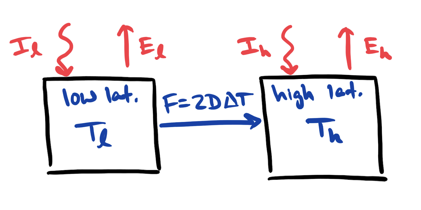
Fig. 6.20 Sketch of a 2-component box model for heat transport.#
The box model that we will use is sketched in Fig. 6.20. We have two boxes - box “l” represents the low latitude (tropical) regions and box “h” represents high latitudes. We assume symmetry about the equator so that the high latitude box represents the combined northern and southern high latitudes. To account for this, the flux of heat from low latitudes to high latitudes, \(F\), is twice what it would be for a single hemisphere. It would be relatively straightforward to use three boxes to represent southern and northern high latitudes in addition to the low latitude box. Indeed, one of the advantages of box models is that they are flexible and can easily be expanded.
Although the exact latitude separating the two boxes is arbitrary, it is common to take it to be about 30\(^\circ\) so that the surface area of the low latitude box and the combined surface area of the high latitudes in the high latitude box are approximately equal. This allows us to use the same heat capacity in each box which keeps things a bit simpler.
The rate of change in the heat content in each box is simply the sum of the incoming and outgoing heat fluxes for that box:
As before, the incoming shortwave radiation is represented by \(I\) and the emitted longwave radiation is represented by \(O\). Subscripts are used to indicate the box where the exchange occurs. As before, the incoming shortwave radiation will be prescribed, but now \(I_l\) and \(I_h\) are simply constants. We will use the same form for the emitted radiation, namely
where \(i=l,h\) and \(T_i\) is the mean temperature in the corresponding box, e.g. \(T_l\) represents the mean temperature in the low latitude box.
We assume that the heat flux, \(F\), is proportional to the difference between the temperatures in the low latitude and high latitude boxes. We will let \(D\) be the coefficient of proportionality and as noted above, we need to multiply by a factor of two to account for the heat flux going south and north from the low latitude box. Hence we take \(F=2D\Delta T\), where \(\Delta T=T_l-T_h\).
Using these forms for \(O\), and \(F\), we have
This represents a system of coupled first order ordinary differential equations. In the first practical project, you will timestep these equations numerically.
Here, we are primarily interested in the equilibrium temperature difference, \(\Delta T\), implied by the model. Steady state solutions require that the LHS of Eq. (6.25) and (6.26) are zero. If we then subtract Eq. (6.26) from Eq. (6.25), we obtain
and hence the equilibrium temperature difference is
Adding Eq. (6.26) to Eq. (6.25), we obtain
Then combining with the expression for \(\Delta T\) ((6.27)) we obtain
Note that each of \(T_h\) and \(T_l\) is determined by a weighted average of \(I_h\) and \(I_l\).
Our last task is to estimate \(D\). First, let’s do this using our estimate for the diffusive heat flux from the last section. Notice that the units of \(D\) are W/m\(^2\)/\(^\circ\)C so that the units of \(DT\) match \(I\) and \(E\). The form of the diffusive heat flux that we used in the last section is
and the units of this are W/m (check this yourself!). Recall that at a state of equilibrium, the diffusive heat flux across a given latitude is equal to the integral of the incoming and outgoing heat fluxes from the equator to that latitude. Therefore, to get a heat flux in units of W/m\(^2\), we need to divide by the approximate north/south width of each box, say \(\pi R_e/2\). Let’s further approximate \(\partial T/\partial y\) with \(\Delta T/(\pi R_e/2)\). Then we can equate the flux in the box model with the approximate diffusive flux:
This gives us the following estimate for \(D\):
using \(\kappa = 5 \times 10^{6} \mbox{m}^2/\mbox{s}\).
Based on Fig. 6.18 (with the low latitude box representing the range from \(-30^\circ\)S to \(30^\circ\)N, we might take \(I_l=280\)W/m\(^2\) and \(I_h=160\)W/m\(^2\). With \(B=2\)W/m\(^2\)/\(^\circ\)C as before, we estimate from Eq. (6.27) that the difference between the low latitude and high latitude temperatures is \(\Delta T \simeq 40^\circ \mbox{C}\). This is comparable to the pole to equator temperature difference and is certainly reasonable given the degree of approximations involved in this model.
The estimate for \(\kappa\) and \(D\) above works relatively well for the modern earth, but what about other planets or past or future climates? When we estimated the diffusivity, \(\kappa\), in the previous section, we used the characteristic velocity and size of weather systems on the modern Earth. On other planets, the wind speed can vary greatly. For example, the winds on Venus can exceed 100 m/s! Clearly this could have a large impact on the heat transport and hence the temperature distribution (and habitability) of a planet. This raises the question: how can we estimate the poleward heat flux in a more general way?
Lorenz et al.\ 2001 (Geophysical Research Letters, 28, 3, 415-418) proposed that dynamics on a planet adapt so that the rate of change in entropy is maximized. While Lorenz et al.\ didn’t provide a firm physical explanation for this hypothesis, they showed that it gives good predictions for the equilibrium temperature on the Earth, Mars, and Titan - planets (and a moon) with very different atmospheres.
The second law of themodynamics states that the change in entropy, \(S\), for a system can be related to the transer of heat into the system, \(Q\) and the temperature, \(T\) according to:
where \(\delta\) denotes a small change. The rate of change of the entropy in each of our boxes is then:
since the heat flux \(F\) is the transfer of heat per unit time. The minus sign is needed in the equation for \(S_l\) since heat is flowing out of this box when \(F>0\). The rate of change in entropy of the full system is then
where \(S=S_l+S_h\). Recall that at equilibrium \(\Delta T=(I_l-I_h)/(4D+B)\) and hence
\(dS/dt\) is maximum when \(D=B/4\) (see example sheet problem). Since \(B\) can be estimated from the chemical and optical properties of the atmosphere (which we know from the paleo record for past climates or spectroscopy for exoplanets), this gives us a powerful tool to estimate the temperature distribution on a planet with limited available measurements.
The 2-box model can be used to illustrate interesting aspects of the climate of the Earth (and of other planets). We consider the example of the ice-albedo effect. As the climate warms, ice melts from the polar regions and mountains. Since ice is very reflective, less ice means that less radiation is reflected from the earth and hence the earth absorbs more solar radiation. This creates a feedback where the earth will warm faster. A similar feedback occurs as the planet cools (e.g. heading into an ice age).
The net incoming SW radiation is the difference between the incident radiation and the fraction reflected directly back to space. For the Earth’s atmosphere some radiation is reflected by clouds and aerosols and some by the surface. We focus on the latter.
The albedo is the fraction of incident SW radiation reflected by the surface. The value of the albedo depends on different characteristics of the surface, e.g. the presence or absence of vegetation. A very important dependence is on ice cover. An ice-covered surface has much larger albedo that a surface without ice.
How does this affect the 2-box calculation. If the surface in the box \(i\) is ice-covered then the net incident SW radiation \((I_i)\) in the calculation above, needs to be multiplied by a factor \(\sigma\) where
But it also needs to be taken into account that ice cover in the box \(i\) is realisable only if the temperature \(T_i\) less that a threshold value \(T_{\rm ice}\) for ice formation.
We assume that \(I_h < I_i\) so that \(T_h < T_l\) implying a state with ice in box \(l\) only is impossible. There are then, in principle, three possible states:
no ice in either box (`ice-free state’)
ice in box \(h\) only (1high-latitude-ice state’)
ice in boxes \(h\) and \(l\) (1global-ice state’).
But only a subset of these states may be realisable (i.e. with \(T_i < T_{\rm ice}\)). Detailed calculation shows that there is always at least one realisable state and sometimes more that one.
We illustrate the behaviour by using the same values of \(A\), \(B\) and \(D\) as before. We set \(\sigma=0.6\) and \(T_{ice}=-10^\circ C\). We introduce a parameter \(q\) representing the relative strength of solar radiation, so that the values of \(I_h\) and \(I_l\) used above are now multiplied by \(q\). We can then calculate the temperatures \(T_h\) and \(T_i\) in each of the three possible states as a function of \(q\) and check whether the state is realisable.
The variation of \(T_l\) and \(T_h\) with \(q\) are shown in Fig. 6.21. The three states, ice free, high latitude ice and global ice, are shown with different line styles. Different states are realisable for different ranges of \(q\). For a given value of \(q\) there may be one, two or three realisable states. This raises the question of, when there is more than one realisable state, which state is actually achieved. This may be addressed by considering the stability of the state (what happens in the time-evolving problem when there is a small perturbation to the steady state), or the effect of slow time variation of \(q\), e.g. what happens if the system starts in an ice-free state with \(q\) large and then \(q\) is slowly reduced?
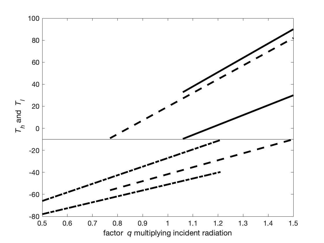
Fig. 6.21 Variation of temperatures \(T_l\) and \(T_h\) with strength of solar radiation. The three states, ice free (solid line), high latitude ice (dashed line) and global ice (dash-dot line), are shown where realisable. For a given line style the upper line shows \(T_l\) and the lower line \(T_h\). A horizontal line shows the threshold value \(T_{\rm ice}\). Different states are realisable for different ranges of \(q\). For a given value of \(q\) there may be one, two or three realisable states.#
There is strong evidence that during periods of its history the Earth has been in (or close to) a global-ice state – `Snowball Earth’. A more sophisticated (but still very simple) model can be formulated using the 1-D approach of Lecture 5. Then the boundary between ice/no ice is at some value of \(y\), \(y_b\) say, which is a function of \(q\).