4.1. Catchment and drainage#
Background#
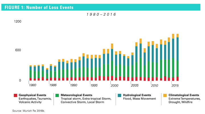
Fig. 4.1 Illustration of the number of major loss events by natural processes, showing the very large proportion of such events associated with flooding.#
Intense floods often lead to severe damage to property, land and infrastructure, and they are becoming one of the main destructive consequences of the more intense rainfall. This is a characteristic of global warming and is compounded by rapid land development which has not maintained adequate water drainage pathways, leading to under-capacity and flooding. Heavy rainfall events have been increasing up over time owing to the higher atmospheric temperatures and the associated capacity for the air to carry more moisture (Fig. 4.2).
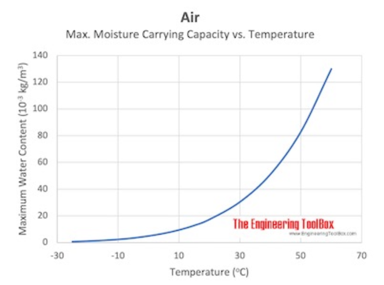
Fig. 4.2 Plot of the water carrying capacity of air at \(100 \ \%\) humidity, as a function of temperature. From The Engineering ToolBox, (2008).#
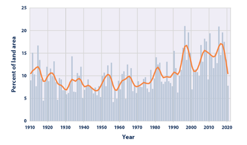
Fig. 4.3 The area of land subjected to heavy rain events every year in the US over time.#
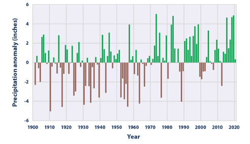
Fig. 4.4 The change in the total annual amount of precipitation in the contiguous 48 states of the USA since 1901. This uses the 1901-2000 average as a baseline for depicted change. Choosing a different baseline period would not change the shape of the pattern over time, but would change the absolute value.#
In the USA, this increase in carrying capacity has led to an increase in land area subject to heavy rainfall (Fig. 4.3), and an overall increase in the average precipitation over the last 90 years (Fig. 4.4) There is a clear trend towards heavier more intense rain and also of increasing annual rainfall.
Rainfall provides the source for much of the flooding inshore, and occurs when the drainage system is unable to accommodate the water flux associated with rain. However, sea level rise will also lead to flooding of near coastal areas, and the two maps below illustrate some predictions of those areas of East Anglia and London which may be submerged by 2100 AD with sea level rise predicted by some climate forecasts (Fig. 4.5).
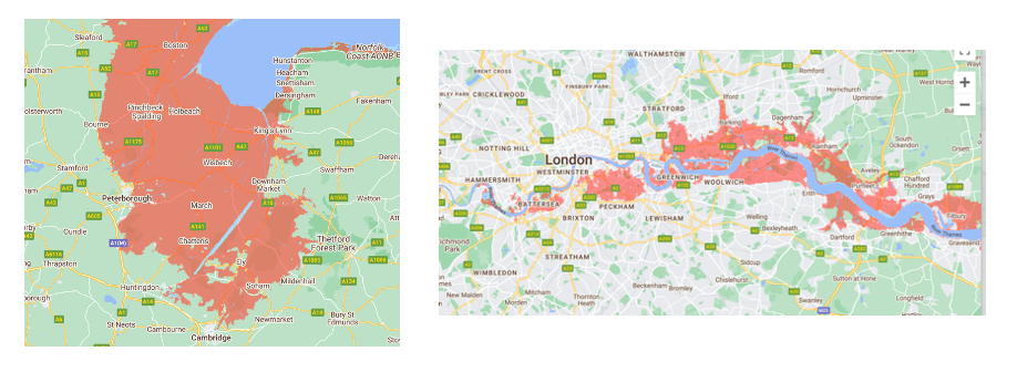
Fig. 4.5 Flooding in East Anglia and London associated with some predictions of sea level rise in the latter part of the present century.#
Rainfall and drainage systems#
Rainfall typically accumulates on the ground and disperses through three pathways. First the rain may run over the land surface downhill towards drainage channels, a process we will call surface run-off, \(S\), with a flux per unit area. Second the rain may infiltrate into the ground, flowing into the subsurface aquifers, a process we label with a flux, \(I\), per unit area. Third, some rainfall is taken up by crops and then returned to the atmosphere by the process of evapotranspiration, with a flux, \(T\), per unit area of the land. The controls on these three fluxes are associated with the type of vegetation, the slope of the land and the type of soil which will be more or less permeable, and hence will regulate the flux of water into the ground. If the surface run-off if too large, then this may lead to overspilling of drainage gullies and channels, and a flood may develop.
Eventually, the drainage and surface run off may reach a river where the flow is localised and moves downstream. If the flow exceeds the river capacity, the flow will overtop the river banks and flood to the flanks of the river, possibly spreading over the flood plain.
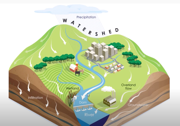
Fig. 4.6 A schmatic showing the flow of water through a watershed scale system.#
Typically, the upstream topography of the land determines the boundaries between different drainage basins,
along lines of maximum elevation known as the watershed.
An example of the Missouri and Mississippi river watersheds in the US is shown in US_river_basins.
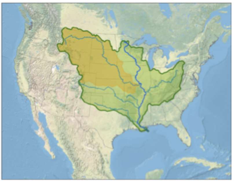
Fig. 4.7 Map showing the watersheds that flow into the Missouri (in yellow) and Mississippi rivers.#
To set the scene for modelling runoff, it is important to assess the volume flux involved in different types of rain event. Light rain may lead to \(0.1 \ \mathrm{mm \ hour^{-1}}\); moderate rain \(1 \ \mathrm{mm \ hour^{-1}}\) and heavy rain may be \(10 \ \mathrm{mm \ hour^{-1}}\). If a river has a catchment area of \(100 \times 100 \ \mathrm{km}\), corresponding to \(10^{10} \ \mathrm{m}^2\) then the volume of rain which falls in 1 hour may range from \(10^7 – 10^9 \ \mathrm{m}^3\). The surface run-off and some drainage fraction of this volume will flow into the river. If the rain fall were to flow directly into the river, it would require a flow rate capacity of about \(3 \times 10^3 - 3 \times 10^5 \ \mathrm{m^3s^{-1}}\). A large river may have a width of \(1000 \ \mathrm{m}\) and depth of \(10 \ \mathrm{m}\), and so the smaller flux could be carried down the river at a speed of about \(0.3 \ \mathrm{m s^{-1}}\) but the larger rainfall event would require a flow rate of \(30 \ \mathrm{m s^{-1}}\) if the rain directly entered the river. Fortunately the drainage system is large and leads to very significant delays in the rain fall reaching the river, as we will now explore. This delay is key to preventing flooding in many cases.
0D model of drainage#
Modelling the drainage of water throughout a catchment area is very complicated. We need to know the capacity of the system to store water and how water flows in and out. On real terrain, the ground may be irregular and so the way in which water flows through it and is stored will be difficult to model.
Given this heterogeneity in the terrain typical in many catchments, it is helpful to first develop an averaged description of the run-off flow from a localised area of the catchment. Eventually, we can add these together as shown in the figure of the multiple drainage zones which flow into the main river.
But first, we therefore work with an integrated picture of the volume of surface water, and relate this to the net run-off flow with a 0D model, with no spatial component. We can consider this a “bucket model” of the drainage basin, as shown in Fig. 4.8.
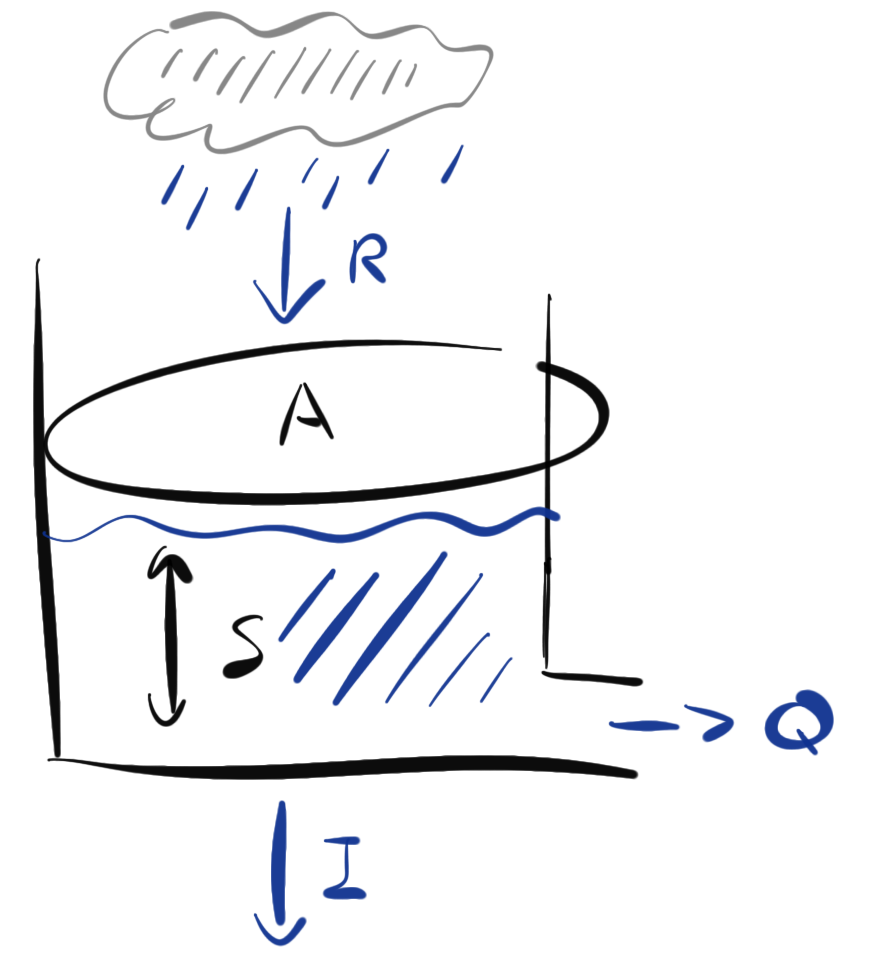
Fig. 4.8 Schematic of the 0D (or “bucket”) model of surface water drainage, over an area \(A\), with an average water depth of \(S\), an input of water due to rainfall at a rate \(R\) per unit area, and fluxes out due to flow into a stream and infiltration (per unit area), \(Q\) and \(I\) respectively.#
In this model we will consider the catchment area as a single bucket that accounts for the surface water stored in the area. This bucket has a single input of water due to rainfall, \(F_{in} = RA\), where \(R\) is the (constant) rainfall rate, and \(A\) is the surface area of the watershed. The volume of water stored in the bucket will be \(V = SA\) where \(S\) is the (averaged) depth of water stored in our conceptual bucket.
The fluxes out of the box will be due to infiltration (per unit area) into the soil, a constant \(I\), and a flux out proportional to the amount stored in the bucket \(Q = \lambda V\), where we have not yet identified our constant of proportionality \(\lambda\).
Balancing the fluxes in and out of the system, we can develop an expression for how the volume stored in the system varies with time
and if we recognise that the surface area of our catchment is constant with time, and dividing through by a factor of that area we get
We have ignored losses due to evapotranspiration, however we could readily include this in the model, provided we have a relation between evapotranspiration and the rain fall. In heavily vegetated zones this would be a significant process, and the vegetation would also impact the value of \(\lambda S\), the surface run-off rate, since it baffles the surface runoff.
We expect that the water flows from the surface into a network of small drainage channels which then coalesce into larger channels, and eventually flow into a tributary. The simple parameterisation is designed to capture the flow over the surface in a simple fashion including the roughness of the surface, the slope and the vegetation. In the example sheet we explore a nonlinear flux law, but the simple model provides a useful framework for interpreting how a simple drainage system operates.
We now develop our simple, 0D model further to find a solution describing how the water stored \(S\), varies in time. Assuming a constant rainfall and infiltration rate, we can apply an integrating factor \(e^{\lambda t}\) to get the solution
where the term \(S(0)\) accounts for the initial volume of water stored in the system.
If the rain is finite in duration (a duration \(T\), for example) then the above solution applies for \(0<t<T\). When the rain stops (i.e. for \(t<T\)), we loose the rainfall term, and are just left with the infiltration and flux out, giving us the form
and in this expression \(S(T)\) is evaluated as in (4.3). Since we have prescribed the surface runoff flow from the land to the river to be \(\lambda S\), by assessing the value of \(S\) at any given time we can evaluate the runoff rate.
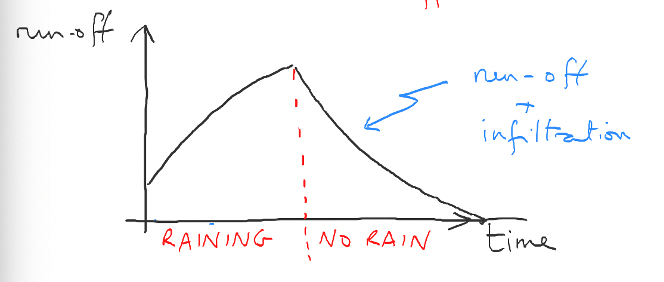
Fig. 4.9 Plot showing the response of the run-off rate to constant rainfall.#